The sentence that says what

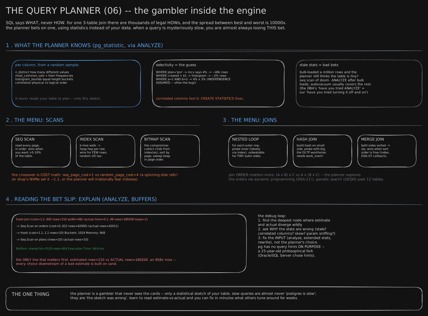
The machine inside a database that turns a question you type into a way of fetching the answer. This lesson is about the question you type; the rest of the chapter opens the machine.

Before you start. You have used an app that saves things: a sign-up form, a bank balance, a list of past orders. That is all this lesson needs; it comes first in the chapter and teaches the language every later lesson reads.

May 1974: a language for accountants and urban planners

In May 1974, at a workshop in Ann Arbor, Michigan, two researchers from IBM’s lab in San Jose, Donald Chamberlin and Raymond Boyce, presented a paper called “SEQUEL: A Structured English Query Language”. Four years earlier their IBM colleague Edgar Codd had proposed keeping data as plain tables, and the San Jose lab was starting to build a database on that idea. What it lacked was a way for people to ask it things.

Their first try, SQUARE, looked like a maths formula and was hard to type. So they started again, in words.

The paper’s first example: Find the names of employees in the toy department. And the answer, in their new language:

SELECT NAME
FROM   EMP
WHERE  DEPT = 'TOY'

The paper says who it was for: people who are “not computer specialists”, and it names them, “accountants, engineers, architects, and urban planners”. It also describes how a person does the job by hand: they “might look down the DEPT column of the EMP table, finding ‘TOY’ entries and making a list of the corresponding NAME entries”. The new sentence says none of that. It names the answer and stops.

Boyce did not see what came of it. He died of an aneurysm in June 1974, a month after the workshop, aged 27. SEQUEL later became SQL, the language nearly every database since has spoken, including Postgres, the free database this chapter opens up.

Ask the librarian: say what, never how

Picture a big library. You can walk the aisles yourself, checking every spine for the author you want. Or you can go to the desk and say: “Every book by Ursula Le Guin, please.” You have said what you want, not how to find it. The librarian knows the building and picks the fastest way.

A database keeps data in tables. A table is a grid: each row is one record (one user), each column is one field of it (a name, a city). This chapter runs on one small database you can build on your laptop in two commands (the second read shows how): a users table with 100,000 rows and an accounts table with 106,667, the same rows on every machine. Here is a question to it, written the way Chamberlin and Boyce wrote theirs:

SELECT id, name, city FROM users WHERE id <= 5;

What the database handed back, from a real run on 2026-09-28:

 id |  name   |   city    
----+---------+-----------
  1 | bob_1   | Pune
  2 | carol_2 | Kolkata
  3 | dev_3   | Pune
  4 | esha_4  | Hyderabad
  5 | farid_5 | Hyderabad
(5 rows)

SELECT names the columns you want, FROM names the table, WHERE says which rows count. A question written this way is a query. Ask how many users live in Pune and the answer is 10,065. The query never said how to find them: walk all 100,000 rows, or jump straight to the Pune ones. That choice was left to the database, the way the shelves were left to the librarian.

Two tables, one answer: the join

Users and accounts live in separate tables. Each row of accounts carries a user_id, the id of the user who owns it, like a borrowing slip carrying a reader’s card number. To see a user beside their accounts, you ask for rows from both tables where that number matches:

flowchart LR
  U["users row: id 3, dev_3"] -->|"accounts.user_id = 3"| A1["account: credit, 17903"]
  U -->|"accounts.user_id = 3"| A2["account: credit, 34384"]
  F["users row: id 5, farid_5"] -.->|"no account has user_id 5"| X["nothing to pair with"]

That pairing is a join. For the first six users it printed seven rows: user 3 twice (two accounts), user 6 twice, and user 5 not at all. The practice data behind these runs was built so that every fifth user has no account, and a plain join shows only pairs that exist. Write LEFT JOIN instead and every user comes back, with farid_5 standing next to an empty slot where the account would be. Which one you want is part of the answer, so SQL makes you say it.

Folding rows into groups: GROUP BY

“How many users live in each city?” is a question about piles, not rows. You tell the database to sort the users into a pile per city and count each pile:

SELECT city, count(*) FROM users GROUP BY city ORDER BY count(*) DESC;

That is GROUP BY: one output row per pile. It printed ten rows. Nine were cities, each with roughly ten thousand users, Delhi on top at 10,185. The tenth row had a count of 9,937 and nothing at all in the city column.

The blank that is not a value: NULL

In 2009, at the QCon conference in London, the computer scientist Tony Hoare gave a talk called “Null References: The Billion Dollar Mistake”. In 1965, designing a programming language called ALGOL W, he had added a way for a slot to hold nothing, “simply because it was so easy to implement”. He guessed it had since caused a billion dollars of errors and crashes. His was a programming language’s nothing, not SQL’s, but SQL’s bites the same way.

Those 9,937 users signed up without giving a city. Their city is not an empty word; it is a slot marked “unknown”, and SQL calls that mark NULL. Now ask a question that must surely cover everyone: users whose city is Pune, or whose city is not Pune. The count came back 90,063, not 100,000.

Here is why. Is an unknown city equal to Pune? The database will not say yes, and it will not say no. It says “unknown”, a third answer beside true and false, and WHERE keeps only the rows that come out true. So every NULL row falls out of both halves of the question, and 9,937 users vanish. The same rule catches city = NULL, which looks like the obvious way to find them and returned 0 rows: nothing is ever known to equal an unknown, not even another unknown. SQL has a separate test for the mark itself, city IS NULL, and that one returned all 9,937.

A librarian holding a book with no author on it would not file it under “not Le Guin” either. She would say she does not know.

Who picks the how: the planner

Every query so far said what it wanted and left the how alone. Something inside the database has to decide it, fresh, for every query. That part is the planner, and it is the librarian of this story.

flowchart TD
  Q["your query: says WHAT"] --> P["the planner: decides HOW"]
  P -->|"one user, by id"| A["jump to that user, then check each account"]
  P -->|"every Pune user"| B["read both tables whole and match them up"]
  A --> R["the rows you asked for"]
  B --> R

Two queries of the same shape show it. Joining users to their accounts for one user by id, the planner went straight to that one user through a lookup the table keeps on its ids. Joining for every Pune user, about 10,000 of them, it read both tables from end to end instead, because touching ten thousand scattered users one at a time would cost more than one pass over everything. Same sentence, two routes, and you asked for neither.

This is where the library stops matching. A librarian learns one building over years and fetches a few books a day. The planner chooses in a moment, for tables of any size, from a short summary of what each table holds; how it guesses, and how it guesses wrong, is the planner lesson later in this chapter. Everything between here and there is the shelving: how rows sit on disk, what is kept close at hand, what makes one route cheaper. You will keep writing the same kind of sentence the whole way through.

You now know

• SQL is a language for asking a database questions; a query names the answer you want and never the steps to find it.
• A join matches rows from two tables on a shared value, such as putting each account beside the user whose id it carries. A plain join leaves out a user with no account; a left join keeps that user and leaves the account columns blank.
• GROUP BY sorts rows into piles by a column and returns one row per pile, such as a count of users per city.
• NULL marks a value as unknown; any comparison with it comes out unknown rather than true or false, so = NULL finds nothing and IS NULL is the test that works.
• Inside the database, a part called the planner picks how to answer each query, and two queries of the same shape can be answered in completely different ways.

Stop here if you want. What follows is the rest of the language in real runs, then twelve exercises on the same two tables, each with its answer.

Second read: every clause, then twelve exercises

Your bench

Every query in this lesson ran on the chapter’s bench: a throwaway Postgres 16 in Docker, filled by a script that makes the same rows on every machine. The Pages and heap files lesson, later in this chapter, uses the same bench and says more about it. Start the database. Docker runs a program in a sealed box on your machine; this line fetches Postgres 16, names the box dbbench, sets its password to bench, and makes it reachable on port 5433 (a numbered door on your machine):

docker run -d --name dbbench -e POSTGRES_PASSWORD=bench -p 5433:5432 postgres:16

Then fill it:

cd teaching/code/di-bench
python3 seed.py

"""Seed the Database Internals bench: one Postgres every Try it in the track runs on.

Creates two tables, dropping them first, so running it again resets them:

  users     100,000 rows  id (primary key), name, email, city, signed_up_at
            city is NULL for about one user in ten.
  accounts  106,667 rows  id (primary key), user_id, kind, balance, opened_at
            users whose id is a multiple of 5 have no account; the rest have
            one, and those whose id is also a multiple of 3 have two.
            kind is 'checking', 'savings' or 'credit'.

Every value is derived from the row number (md5 of it, and modulo), never
random(), so every reader's bench holds the same rows. The only indexes are
the two primary keys, users_pkey and accounts_pkey, plus nothing on
accounts.user_id on purpose: a missing index has to show up somewhere.

Run it against a postgres:16 container (the name defaults to dbbench):

  docker run -d --name dbbench -e POSTGRES_PASSWORD=bench -p 5433:5432 postgres:16
  python3 seed.py            # or: python3 seed.py <container-name>

Python 3 standard library only. It pipes SQL into psql inside the container
with `docker exec -i <container> psql -U postgres`.
"""

import subprocess
import sys
import time

CONTAINER = sys.argv[1] if len(sys.argv) > 1 else "dbbench"
USERS = 100_000

# h(x) is a 32-bit number read off md5(x): the same on every machine, every run.
SEED_SQL = f"""
DROP TABLE IF EXISTS accounts;
DROP TABLE IF EXISTS users;

CREATE TABLE users (
    id           int         NOT NULL,
    name         text        NOT NULL,
    email        text        NOT NULL,
    city         text,
    signed_up_at timestamptz NOT NULL
);

INSERT INTO users (id, name, email, city, signed_up_at)
SELECT g,
       n.first || '_' || g,
       n.first || '_' || g || '@example.com',
       (ARRAY['Pune', 'Delhi', 'Mumbai', 'Bengaluru', 'Chennai',
              'Kolkata', 'Jaipur', 'Hyderabad', 'Lucknow', NULL])[1 + h.v % 10],
       timestamptz '2024-01-01 00:00:00+00'
         + (h.v % 1000) * interval '1 day'
         + (g % 1440)   * interval '1 minute'
FROM generate_series(1, {USERS}) AS g
CROSS JOIN LATERAL (
    SELECT ('x' || substr(md5(g::text), 1, 8))::bit(32)::bigint AS v
) AS h
CROSS JOIN LATERAL (
    SELECT (ARRAY['alice', 'bob', 'carol', 'dev', 'esha',
                  'farid', 'gita', 'hari'])[1 + g % 8] AS first
) AS n
ORDER BY g;

ALTER TABLE users ADD CONSTRAINT users_pkey PRIMARY KEY (id);

CREATE TABLE accounts (
    id        int         NOT NULL,
    user_id   int         NOT NULL,
    kind      text        NOT NULL,
    balance   int         NOT NULL,
    opened_at timestamptz NOT NULL
);

INSERT INTO accounts (id, user_id, kind, balance, opened_at)
SELECT row_number() OVER (ORDER BY u.id, k),
       u.id,
       (ARRAY['checking', 'savings', 'credit'])[1 + h.v % 3],
       (h.v % 50000)::int,
       u.signed_up_at + (h.v % 90) * interval '1 day'
FROM users AS u
CROSS JOIN LATERAL generate_series(
    1,
    CASE WHEN u.id % 5 = 0 THEN 0      -- no account at all
         WHEN u.id % 3 = 0 THEN 2      -- two accounts
         ELSE 1 END
) AS k
CROSS JOIN LATERAL (
    SELECT ('x' || substr(md5('acct' || u.id || '-' || k), 1, 8))::bit(32)::bigint AS v
) AS h
ORDER BY u.id, k;

ALTER TABLE accounts ADD CONSTRAINT accounts_pkey PRIMARY KEY (id);
ALTER TABLE accounts ADD CONSTRAINT accounts_user_id_fkey
    FOREIGN KEY (user_id) REFERENCES users (id);

VACUUM ANALYZE users;
VACUUM ANALYZE accounts;
"""

SUMMARY_SQL = """
SELECT label, n FROM (
          SELECT 1 AS ord, 'users' AS label, count(*) AS n FROM users
UNION ALL SELECT 2, 'accounts', count(*) FROM accounts
UNION ALL SELECT 3, 'users with no account', count(*) FROM users u
          WHERE NOT EXISTS (SELECT 1 FROM accounts a WHERE a.user_id = u.id)
UNION ALL SELECT 4, 'users with city NULL', count(*) FROM users WHERE city IS NULL
UNION ALL SELECT 5, 'accounts, kind = ' || kind, count(*) FROM accounts GROUP BY kind
) s ORDER BY ord, label;
"""


def psql(sql, *flags):
    return subprocess.run(
        ["docker", "exec", "-i", CONTAINER,
         "psql", "-U", "postgres", "-X", "-v", "ON_ERROR_STOP=1", *flags],
        input=sql, text=True, capture_output=True,
    )


def wait_for_postgres():
    # The image starts a temporary server to initialise, then restarts. The
    # temporary one does not listen on TCP, so asking over 127.0.0.1 waits
    # for the real one.
    for _ in range(60):
        r = subprocess.run(
            ["docker", "exec", CONTAINER, "pg_isready", "-h", "127.0.0.1", "-U", "postgres"],
            capture_output=True, text=True,
        )
        if r.returncode == 0:
            return
        time.sleep(1)
    sys.exit(f"Postgres in container {CONTAINER!r} did not come up in 60s")


def main():
    wait_for_postgres()
    r = psql(SEED_SQL, "-q")
    if r.returncode != 0:
        sys.exit(r.stderr)
    r = psql(SUMMARY_SQL, "-At", "-F", "\t")
    if r.returncode != 0:
        sys.exit(r.stderr)
    print("bench seeded:")
    for line in r.stdout.splitlines():
        label, count = line.split("\t")
        print(f"  {label:<26} {int(count):>7,}")


if __name__ == "__main__":
    main()

What it printed (measured 2026-09-28, on a fresh container):

bench seeded:
  users                      100,000
  accounts                   106,667
  users with no account       20,000
  users with city NULL         9,937
  accounts, kind = checking   35,544
  accounts, kind = credit     35,261
  accounts, kind = savings    35,862

users has id, name, email, city (NULL for about one user in ten) and signed_up_at. accounts has id, user_id, kind (checking, savings or credit), balance and opened_at. Users whose id is a multiple of 5 have no account; the rest have one, and those whose id is also a multiple of 3 have two. Open a prompt with:

docker exec -it dbbench psql -U postgres

Then type \pset null '(null)' once. Postgres prints NULL as blank by default, which is how the story’s GROUP BY row looked empty; with this setting it prints (null), and every output below except the city count was captured with it on. docker rm -f dbbench throws the bench away when you are done.

The clauses, in the order the database reads them

You write SELECT … FROM … WHERE … GROUP BY … HAVING … ORDER BY … LIMIT. The database reads them in a different order: FROM (and any join), then WHERE, then GROUP BY, then HAVING, then SELECT, then ORDER BY, then LIMIT. That order explains most of the rules below. WHERE runs before the piles exist, so it cannot filter on a count; HAVING runs after, so it can.

The story’s plain join, for the first six users. Each row is one user paired with one of their accounts; user 5 is missing:

SELECT u.id, u.name, a.kind, a.balance
FROM users u JOIN accounts a ON a.user_id = u.id
WHERE u.id <= 6 ORDER BY u.id, a.id;

 id |  name   |   kind   | balance 
----+---------+----------+---------
  1 | bob_1   | savings  |   27304
  2 | carol_2 | savings  |    6529
  3 | dev_3   | credit   |   17903
  3 | dev_3   | credit   |   34384
  4 | esha_4  | savings  |    7676
  6 | gita_6  | checking |     233
  6 | gita_6  | checking |   27549
(7 rows)

The same with LEFT JOIN. Farid has no account, so his account columns are NULL:

SELECT u.id, u.name, a.kind, a.balance
FROM users u LEFT JOIN accounts a ON a.user_id = u.id
WHERE u.id <= 6 ORDER BY u.id, a.id;

 id |  name   |   kind   | balance 
----+---------+----------+---------
  1 | bob_1   | savings  |   27304
  2 | carol_2 | savings  |    6529
  3 | dev_3   | credit   |   17903
  3 | dev_3   | credit   |   34384
  4 | esha_4  | savings  |    7676
  5 | farid_5 | (null)   |  (null)
  6 | gita_6  | checking |     233
  6 | gita_6  | checking |   27549
(8 rows)

The story’s city count, every pile, captured before \pset null was set; the blank-city pile is the seventh row:

   city    | count 
-----------+-------
 Delhi     | 10185
 Lucknow   | 10100
 Bengaluru | 10089
 Kolkata   | 10086
 Pune      | 10065
 Jaipur    |  9948
           |  9937
 Hyderabad |  9898
 Mumbai    |  9852
 Chennai   |  9840
(10 rows)

ORDER BY and LIMIT. A table has no order of its own; without ORDER BY, rows come back in whatever order the chosen route produced them, and that can change. ORDER BY sorts, LIMIT keeps the first few. The five biggest balances, ties broken by account id:

SELECT id, user_id, kind, balance FROM accounts ORDER BY balance DESC, id LIMIT 5;

  id   | user_id |   kind   | balance 
-------+---------+----------+---------
 72053 |   67549 | savings  |   49999
 31711 |   29728 | checking |   49998
 89208 |   83632 | savings  |   49998
 92148 |   86388 | savings  |   49998
   751 |     703 | credit   |   49997
(5 rows)

GROUP BY with more than a count. Each pile can be summarised any way: count, sum, avg, min, max. Columns read pile, how many accounts in it, their average balance rounded to a whole number:

SELECT kind, count(*) AS accounts, avg(balance)::int AS avg_balance
FROM accounts GROUP BY kind ORDER BY kind;

   kind   | accounts | avg_balance 
----------+----------+-------------
 checking |    35544 |       24940
 credit   |    35261 |       24830
 savings  |    35862 |       25068
(3 rows)

HAVING filters piles. Cities whose users hold more than 10,700 accounts between them:

SELECT u.city, count(*) AS accounts
FROM users u JOIN accounts a ON a.user_id = u.id
GROUP BY u.city HAVING count(*) > 10700 ORDER BY accounts DESC;

  city   | accounts 
---------+----------
 Delhi   |    10895
 Pune    |    10823
 Lucknow |    10782
 Kolkata |    10721
(4 rows)

NULL, three more ways it bites

The three answers. Each column below is one comparison; t is true, and (null) here is the answer “unknown”:

SELECT NULL = NULL AS equal, NULL IS NULL AS is_null,
       1 = NULL AS one_eq_null, NOT (1 = NULL) AS negated;

 equal  | is_null | one_eq_null | negated 
--------+---------+-------------+---------
 (null) | t       | (null)      | (null)
(1 row)

Not-unknown is still unknown. That is why “Pune or not Pune” lost 9,937 rows: city <> 'Pune' alone returned 79,998, which is 100,000 − 10,065 Pune − 9,937 unknown (checked with python3).

COUNT(*) and COUNT(column) are different questions. count(*) counts rows. count(city) counts rows whose city is not NULL:

SELECT count(*) AS every_row, count(city) AS rows_with_a_city FROM users;

 every_row | rows_with_a_city 
-----------+------------------
    100000 |            90063
(1 row)

NOT IN with a NULL in the list returns nothing. city NOT IN ('Pune', 'Delhi') returned 69,813. Add a NULL to the list and it returned 0:

SELECT count(*) FROM users WHERE city NOT IN ('Pune', 'Delhi', NULL);

 count 
-------
     0
(1 row)

NOT IN (a, b, NULL) means “not a, and not b, and not unknown”. The last part is unknown for every row, so no row comes out true. In practice the NULL arrives from a subquery (a query inside another query) over a column that allows NULL; NOT EXISTS or a LEFT JOIN … IS NULL does not have this trap.

Naming a step: WITH

A CTE (common table expression) gives a query’s result a name, so the next step can read it like a table. First each user’s total balance, then how many totals pass 60,000:

WITH totals AS (
  SELECT user_id, sum(balance) AS total FROM accounts GROUP BY user_id
)
SELECT count(*) AS users_over_60k FROM totals WHERE total > 60000;

 users_over_60k 
----------------
           8595
(1 row)

It says nothing about how. The planner is free to run it as one piece.

A window: ranking without folding

GROUP BY folds a pile into one row. A window function computes across a set of rows and keeps every row. rank() OVER (ORDER BY balance DESC) gives each account its place among the others; here, the accounts of users 1 to 12:

SELECT user_id, kind, balance, rank() OVER (ORDER BY balance DESC) AS place
FROM accounts WHERE user_id <= 12 ORDER BY place;

 user_id |   kind   | balance | place 
---------+----------+---------+-------
      11 | checking |   38460 |     1
       3 | credit   |   34384 |     2
      12 | savings  |   29168 |     3
       6 | checking |   27549 |     4
       1 | savings  |   27304 |     5
       9 | savings  |   26397 |     6
       7 | savings  |   25946 |     7
       9 | checking |   24564 |     8
      12 | checking |   18818 |     9
       3 | credit   |   17903 |    10
       4 | savings  |    7676 |    11
       8 | savings  |    7239 |    12
       2 | savings  |    6529 |    13
       6 | checking |     233 |    14
(14 rows)

Add PARTITION BY kind inside the OVER and the ranking restarts for each kind; exercise 10 does that.

The how, printed

EXPLAIN in front of a query prints the planner’s chosen route instead of running it. The story’s two joins. Every Pune user: read both tables whole (Seq Scan), build a lookup of the Pune users in memory (Hash), and match accounts against it (Hash Join):

EXPLAIN SELECT u.name, a.balance FROM users u JOIN accounts a ON a.user_id = u.id WHERE u.city = 'Pune';

                                QUERY PLAN                                 
---------------------------------------------------------------------------
 Hash Join  (cost=2406.34..4538.02 rows=10781 width=15)
   Hash Cond: (a.user_id = u.id)
   ->  Seq Scan on accounts a  (cost=0.00..1851.67 rows=106667 width=8)
   ->  Hash  (cost=2280.00..2280.00 rows=10107 width=15)
         ->  Seq Scan on users u  (cost=0.00..2280.00 rows=10107 width=15)
               Filter: (city = 'Pune'::text)
(6 rows)

One user by id: jump to it through the primary key’s index (Index Scan using users_pkey), then check accounts for its id (Nested Loop):

EXPLAIN SELECT u.name, a.balance FROM users u JOIN accounts a ON a.user_id = u.id WHERE u.id = 42;

                                   QUERY PLAN                                    
---------------------------------------------------------------------------------
 Nested Loop  (cost=0.29..2126.66 rows=1 width=15)
   ->  Index Scan using users_pkey on users u  (cost=0.29..8.31 rows=1 width=15)
         Index Cond: (id = 42)
   ->  Seq Scan on accounts a  (cost=0.00..2118.34 rows=1 width=8)
         Filter: (user_id = 42)
(5 rows)

The rows= figures are the planner’s guesses from a random sample of the table (10,107 Pune users guessed; 10,065 real), so your run may print slightly different guesses and costs. The shape of each plan is the part that should match. Notice the second plan still reads all of accounts to find user 42’s rows: the bench deliberately has no index on accounts.user_id. Reading plans like these is the planner lesson’s job.

Twelve exercises

Each is a question you can answer with what is above. Write your query, run it on the bench, then open the answer. Every answer was run on the bench on 2026-09-28 with \pset null '(null)' on.

1. How many users live in Mumbai?

SELECT count(*) FROM users WHERE city = 'Mumbai';

 count 
-------
  9852
(1 row)

2. The five users who signed up most recently: id, name, sign-up time.

SELECT id, name, signed_up_at FROM users ORDER BY signed_up_at DESC, id LIMIT 5;

  id   |    name     |      signed_up_at      
-------+-------------+------------------------
  4304 | alice_4304  | 2026-09-26 23:44:00+00
 71948 | esha_71948  | 2026-09-26 23:08:00+00
 96378 | carol_96378 | 2026-09-26 22:18:00+00
 11413 | farid_11413 | 2026-09-26 22:13:00+00
 63247 | hari_63247  | 2026-09-26 22:07:00+00
(5 rows)

3. For each kind of account, how many hold more than 40,000?

SELECT kind, count(*) FROM accounts WHERE balance > 40000 GROUP BY kind ORDER BY kind;

   kind   | count 
----------+-------
 checking |  7063
 credit   |  6922
 savings  |  7266
(3 rows)

4. How many users have no account at all?

SELECT count(*) FROM users u LEFT JOIN accounts a ON a.user_id = u.id WHERE a.id IS NULL;

 count 
-------
 20000
(1 row)

5. How many users have exactly two accounts?

SELECT count(*) FROM (
  SELECT user_id FROM accounts GROUP BY user_id HAVING count(*) = 2
) AS two;

 count 
-------
 26667
(1 row)

6. Total balance held by each city’s users, biggest first, with the no-city users labelled.

SELECT coalesce(u.city, '(no city)') AS city, sum(a.balance) AS total
FROM users u JOIN accounts a ON a.user_id = u.id
GROUP BY u.city ORDER BY total DESC;

   city    |   total   
-----------+-----------
 Delhi     | 271600877
 Pune      | 271101090
 Lucknow   | 269134849
 Jaipur    | 265729188
 Bengaluru | 264733192
 Kolkata   | 264651402
 Mumbai    | 264615045
 (no city) | 264505917
 Hyderabad | 264156377
 Chennai   | 260774961
(10 rows)

7. Pune has 10,065 users and Delhi 10,185. Why does WHERE city NOT IN ('Pune', 'Delhi') return 69,813 and not 79,750? Fix it.

SELECT count(*) FROM users WHERE city NOT IN ('Pune', 'Delhi') OR city IS NULL;

 count 
-------
 79750
(1 row)

8. How many users signed up during 2025?

SELECT count(*) FROM users
WHERE signed_up_at >= '2025-01-01' AND signed_up_at < '2026-01-01';

 count 
-------
 36457
(1 row)

9. Among users whose accounts total more than 60,000, which three cities have the most?

WITH totals AS (
  SELECT user_id, sum(balance) AS total FROM accounts GROUP BY user_id
)
SELECT u.city, count(*) AS rich_users
FROM totals t JOIN users u ON u.id = t.user_id
WHERE t.total > 60000
GROUP BY u.city ORDER BY rich_users DESC LIMIT 3;

  city  | rich_users 
--------+------------
 Delhi  |        901
 (null) |        893
 Pune   |        878
(3 rows)

10. The two biggest accounts of each kind.

WITH ranked AS (
  SELECT kind, id, balance,
         rank() OVER (PARTITION BY kind ORDER BY balance DESC) AS place
  FROM accounts
)
SELECT kind, id, balance, place FROM ranked WHERE place <= 2 ORDER BY kind, place, id;

   kind   |  id   | balance | place 
----------+-------+---------+-------
 checking | 31711 |   49998 |     1
 checking | 64608 |   49997 |     2
 credit   |   751 |   49997 |     1
 credit   | 52866 |   49992 |     2
 savings  | 72053 |   49999 |     1
 savings  | 89208 |   49998 |     2
 savings  | 92148 |   49998 |     2
(7 rows)

11. For users 1 to 4, each account next to that user’s total, without losing the account rows.

SELECT user_id, kind, balance, sum(balance) OVER (PARTITION BY user_id) AS user_total
FROM accounts WHERE user_id <= 4 ORDER BY user_id, id;

 user_id |  kind   | balance | user_total 
---------+---------+---------+------------
       1 | savings |   27304 |      27304
       2 | savings |    6529 |       6529
       3 | credit  |   17903 |      52287
       3 | credit  |   34384 |      52287
       4 | savings |    7676 |       7676
(5 rows)

12. Sign-ups per month for January to June 2024, with a running total.

WITH monthly AS (
  SELECT date_trunc('month', signed_up_at)::date AS month, count(*) AS signups
  FROM users WHERE signed_up_at < '2024-07-01' GROUP BY 1
)
SELECT month, signups, sum(signups) OVER (ORDER BY month) AS running_total
FROM monthly ORDER BY month;

   month    | signups | running_total 
------------+---------+---------------
 2024-01-01 |    3119 |          3119
 2024-02-01 |    2906 |          6025
 2024-03-01 |    2964 |          8989
 2024-04-01 |    2902 |         11891
 2024-05-01 |    3072 |         14963
 2024-06-01 |    3001 |         17964
(6 rows)

Try it

1. Build the bench from the second read (two commands, about a minute) and run the twelve exercises before opening any answer.
2. Break a join on purpose: write the users-to-accounts join and leave off the ON a.user_id = u.id, replacing it with ON true, for u.id <= 3 only. Count the rows and explain the number from the table sizes.
3. Put EXPLAIN in front of exercise 4 and exercise 9. Name the operator at the top of each plan. Then run CREATE INDEX ON accounts (user_id);, run EXPLAIN on the one-user join from the second read again, and see which line changed. python3 seed.py rebuilds both tables without the index when you are done.
4. Rewrite exercise 4 with NOT EXISTS and with NOT IN (SELECT user_id FROM accounts). All three should agree here. Say why NOT IN is safe on this column (hint: accounts.user_id is declared NOT NULL) and would not be on users.city.
5. docker rm -f dbbench when you are done.

Go deeper

• Chamberlin and Boyce, “SEQUEL: A Structured English Query Language” (1974) (sixteen pages; the toy-department query is on the first page of examples)
• Postgres tutorial: The SQL Language (joins, aggregates, the basics, from the source)
• Postgres docs: Window Functions tutorial
• Postgres docs: Comparison Functions and Operators (NULL and IS DISTINCT FROM)
• Tony Hoare, “Null References: The Billion Dollar Mistake”, QCon London 2009
• CMU 15-445, Modern SQL lecture - Andy Pavlo (the second lecture of the course, and its first homework).

Related

Database Internals - the deep-dive set · Pages & Heap Files · The Query Planner

The full Database Internals list is in CURRICULUM.

Retrieval practice

7 questions. Answer each one before you open it.