Complexity & Big-O
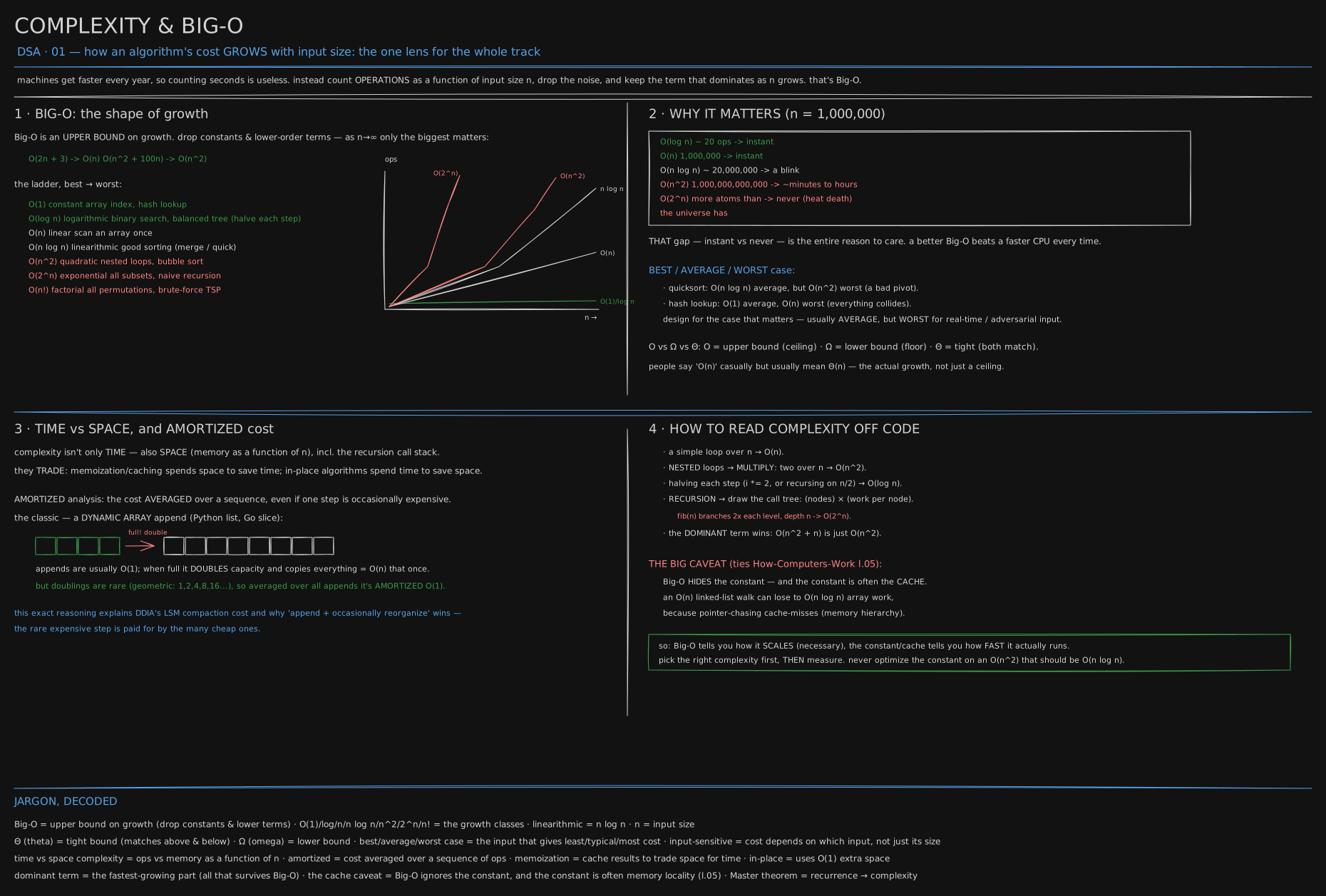
The ladder you’ll use for every data structure and algorithm that follows in this track, and it plugs straight into The Memory Hierarchy (cache, locality, the memory wall).
Before you start. You need to be able to multiply two numbers and read a simple table - that’s the whole of the maths in the story half. This is the first lesson in the DSA track, so there’s nothing earlier to recall. If a cache miss is new, The Memory Hierarchy (cache, locality, the memory wall) in How Computers Work shows it in one read.
1894: a mathematician needs a word for “grows about this fast”
Paul Bachmann was a German number theorist. His problem had nothing to do with computers: he was studying how prime numbers are scattered among all the other numbers, and nobody had an exact formula for how many primes sit below some number n. Nobody has one today either. What mathematicians could do was estimate, and say how good the estimate was - “the gap between my guess and the truth grows no faster than this other, simpler function, once numbers get big enough.”
That phrase needed a shorthand. In 1894, Bachmann started writing the letter O in front of the simpler function to mean exactly that: grows no faster than this. Fifteen years later, in 1909, another number theorist, Edmund Landau, took the notation further in his own work on how primes are distributed - which is why the family of symbols this letter belongs to is still called Bachmann–Landau notation today.
You will not be asked about prime numbers in a coding interview. This is the story of how a 130-year-old shorthand for “roughly this fast” ended up on your whiteboard instead.
1976: the letter means three different things, so Knuth writes a letter
By the 1960s, people writing about programs had borrowed Bachmann’s O for something new: not how far a guess about primes drifts, but how many steps a program takes as you hand it more data to chew through. The trouble was that papers disagreed about exactly what O promised, and about its two cousins - one symbol for a floor under the growth, one for a claim that ties the floor and the ceiling together.
In 1976, Donald Knuth, already famous for The Art of Computer Programming, wrote a short piece for the newsletter SIGACT News called “Big Omicron and Big Omega and Big Theta,” pinning down all three for programmers specifically: one for “no worse than,” one for “no better than,” one for “exactly this, both ways.” His version is the one taught today, and every “O(n)” you will type for the rest of your career is a direct descendant of that fix.
The idea: stop timing it, start counting the shape
Here is the problem timing solves badly. Two programs each take one second on your laptop - which is better? You cannot tell, and running them a third and fourth time will not tell you either. A second on a five-year-old laptop and a second on this year’s is a different amount of work, and next year’s laptop will make both look instant. What buying a new laptop never changes is the shape: does the work double when the data doubles? Quadruple? Barely move at all? Big-O never asks how fast your machine is; it only asks how the pile of work grows as the pile of data grows. That shape is the same on every machine that will ever exist, including ones that have not been built yet.
The front-desk line: five shapes of getting slower
This is also exactly what an interviewer is listening for when they ask “what’s the time complexity of your solution?” They are not asking for a number of seconds. They want the shape: name it (the short names come in a moment) and you have told them exactly how your solution behaves at scale, in four characters, without running a single line. Picture a receptionist looking for one visitor’s name in a line of n people.
If the receptionist already knows exactly where that visitor stands - always at the front, say - finding them takes one check no matter how long the line gets. Ten people, one check. A million people, one check. A shape that does not grow at all is called O(1), constant time.
Now the line is sorted by name. Ask “before the middle or after it?”, throw away the half that cannot hold the name, and repeat on what is left. Ten people takes about three questions. A million people takes about twenty. Every time the line gets ten times longer, this shape only earns a few more questions. That is O(log n), logarithmic.
Unsort the line. The receptionist checks every face, one at a time, until the name turns up. Ten people, ten checks. A million people, a million checks. Double the line and this shape doubles exactly with it: O(n), linear.
Now the receptionist is checking every person against every other person - hunting for a matching pair, say. Ten people is about a hundred comparisons, ten checks for each of ten; a hundred people is ten thousand. Double the line and the work goes up by four. That is O(n²), quadratic.
And if the receptionist had to try every possible group that could be picked from the line, each person either in or out, then every extra person doubles the count. Forty people make about 1.1 trillion groups. Sixty make about a billion billion. That shape is O(2ⁿ), exponential, and it is the one shape you actively fight in an interview.
flowchart LR
  A["10 people in line"] -->|"line doubles to 20"| B["20 people in line"]
  A -->|"O(1): 1 check"| R1["1 check either way"]
  B -->|"O(1): 1 check"| R1
  A -->|"O(n): 10 checks"| R2["10 checks"]
  B -->|"O(n): 20 checks"| R3["20 checks"]
  A -->|"O(n²): 100 checks"| R4["100 checks"]
  B -->|"O(n²): 400 checks"| R5["400 checks"]
Every one of these five shapes turns up again and again in the rest of this track. Naming which shape a piece of code belongs to, before you have even run it, is most of what a coding interview is actually testing. Two more shapes sit on the same ladder - one between O(n) and O(n²), one worse than O(2ⁿ) - and the second read lists all seven and times five of them on a real machine, so the gap between “instant” and “never finishes” stops being a claim and becomes something you can watch a clock make.
You now know
- Big-O describes the shape of how work grows as the input
ngrows, not how many seconds something takes on any one machine. - O(1) does not grow at all. O(log n) barely grows. O(n) grows exactly as fast as the input. O(n²) grows by the square. O(2ⁿ) explodes.
- The same shape can still run at wildly different real speeds on the same machine - that is the constant Big-O throws away, and the second read measures it directly.
Stop here if you want. What follows is the same five shapes, measured on a real machine, with the code that produced every number.
Second read: the five shapes, measured
Formally: count operations as a function of n, drop constants and lower-order terms, keep the fastest-growing term:
O(2n + 3)      → O(n)
O(n² + 100n)   → O(n²)
Big-O is the ceiling; Omega is the floor; Theta is both at once, the tight bound. People say “O(n)” casually but usually mean Theta(n), the actual growth, not merely a ceiling.
The ladder, best to worst (TSP, in the last row, is the travelling salesman problem: the shortest round trip through a list of cities):
O(1)        constant      array index, hash lookup
O(log n)    logarithmic   binary search, balanced tree (halve each step)
O(n)        linear        scan an array once
O(n log n)  linearithmic  good sorting (merge / quick)
O(n²)       quadratic     nested loops, bubble sort
O(2ⁿ)       exponential   all subsets, naive recursion
O(n!)       factorial     all permutations, brute-force TSP
Plotted, these curves diverge violently - shape matters far more than any constant once n is large.
Why it matters, at a million: roughly how many steps each shape needs for a million items.
O(log n)    ~ 20 operations              → instant
O(n)        1,000,000                    → instant
O(n log n)  ~ 20,000,000                 → a blink
O(n²)       1,000,000,000,000            → minutes to hours
O(2ⁿ)       more atoms than the universe → never (heat death)
That gap is why “make it O(n log n) instead of O(n²)” beats any micro-optimization.
Where the 20 and the “atoms” come from, by hand:
 2^10 =           1,024  ≈ 10^3      "ten halvings is a thousand"
 2^20 =       1,048,576  ≈ 10^6      so log2(1,000,000) ≈ 20    (exact: 19.93)
 2^30 =   1,073,741,824  ≈ 10^9      thirty halvings is a billion
 2^40 ≈ 1.1 × 10^12                  forty is a trillion
Ten halvings buys a factor of a thousand, so the log of any n is about 3.3 × its digit count: a million, seven digits, about 20 halvings. Then n log n = 10^6 × 20 = 2 × 10^7, the twenty million above. And 2^1,000,000 ≈ 10^301,030, a number with three hundred thousand digits, against the universe’s roughly 10^80 atoms - not bigger than the atoms, just more ink than the atoms would take to write.
The ladder, timed on this machine. Node (v22), sorted arrays, n rising by ten each row. O(1)/O(log n) time a thousand lookups, since one is too fast to clock; ignore row one, where JIT warm-up shows.
| n | O(1), 1000 index reads | O(log n), 1000 binary searches | O(n) scan | O(n log n) sort | O(n²) nested loops |
|---|---|---|---|---|---|
| 1,000 | 33 us | 427 us | 24 us | 473 us | 1.3 ms |
| 10,000 | 10 us | 66 us | 78 us | 3.8 ms | 51.7 ms |
| 100,000 | 10 us | 79 us | 780 us | 37.6 ms | skipped |
| 1,000,000 | 26 us | 144 us | 7.5 ms | 434 ms | skipped |
O(1) does not move: noise around 10-26 us. O(log n) barely moves, 20 steps at a million. O(n) climbs by ten each row. O(n log n) climbs a touch faster (3.8 → 37.6 → 434, about ×11.5), log n showing itself. O(n²) climbs by a hundred: from 51.7 ms at 10,000, that is 5.2 seconds at 100,000 and 1.4 hours at 1,000,000, why those cells are empty.
Two numbers worth keeping: a thousand binary searches at a million finish in 144 us, faster than one linear scan (7.5 ms), because the sorted array already paid the sort cost. And the sort itself (434 ms) is 58 times the scan, not 20 times as log n alone suggests, since sorting moves data and scanning only reads it - the constant Big-O drops is real, and here it is about three.
Amortized: counted, then timed. A dynamic array starts at capacity 1 and doubles whenever an append does not fit.
10^6 appends with doubling: 20 regrowths, 1,048,575 elements copied in total = 1.05 copies per append
10^6 pushes measured: 5.2 ms -> 5 ns per push
Twenty regrowths, at sizes 1, 2, 4, … 524,288, copy 1 + 2 + 4 + … + 2^19 = 2^20 − 1 = 1,048,575 elements total, and the copying never exceeds 2n - spread over a million appends, about one copy each. That is “amortized O(1)”: rare expensive regrowths, paid for by the many cheap appends around them. A push measures 5 ns; the regrowths are invisible inside that. Python’s list grows by ×1.125 instead of doubling, and measured 36 ns per append over five million - same shape, bigger constant.
The cache caveat, measured. Sum a million integers once from a contiguous array, once by following next pointers through the same count of objects linked in shuffled order. Both O(n), one addition per element.
O(n) sum of 10^6: contiguous array 1.6 ms vs shuffled linked list 63.2 ms -> 39x slower, same Big-OThat 39x is the memory hierarchy from The Memory Hierarchy (cache, locality, the memory wall): the array arrives in cache lines the prefetcher can guess ahead of the loop, the list takes a cache miss on nearly every node. Link the same nodes in allocation order and the sum falls to about 5 ms, a twelvefold difference from layout alone. Big-O picks the class; the constant decides the race.
Reading the shape off a piece of code, as the questions to ask in order:
flowchart TD
    A[look at the loop or the recursion] --> B{does it halve the problem each step?}
    B -->|yes| L[O log n: binary search, tree descent]
    B -->|no| C{one loop over n?}
    C -->|yes, and each step is O 1| N[O n: a scan]
    C -->|yes, with a log n step inside| NL[O n log n: sort, heap per element]
    C -->|nested loop over n| Q[O n squared: every pair]
    C -->|no, it recurses| R{how many calls per level, how deep?}
    R -->|2 calls, depth n| E[O 2 to the n: subsets, naive fib]
    R -->|1 call, depth log n| L
Follow “halve” first: it is the shape binary search (Clinic #11 - Binary Search) and every balanced tree share. Recursion holds the exponential rung; the fix (Clinic #03 - Coin Change, Foundations #02 - Recursion → Memo → Table (DP ka engine)) is to stop the call tree repeating itself.
A few more distinctions worth holding:
- Best / average / worst depends on which input. Quicksort is O(n log n) average, O(n²) on a pathological pivot; a hash lookup is O(1) average, O(n) if everything collides.
- Space, not just time. Complexity also counts memory as a function of
n, call-stack depth included - the reasoning behind every “append cheaply, reorganize rarely” design. - The dominant term wins: O(n² + n) is O(n²); a call tree is node count times work per node, so
fib(n)’s two calls per level overnlevels gives O(2ⁿ).
Try it
Feel the divergence and the amortization empirically:
import time
def cost(fn, n):
    t = time.perf_counter(); fn(n); return time.perf_counter() - t

def quad(n):
    for i in range(n):
        for j in range(n): pass                 # O(n^2)
for n in [1000, 2000, 4000]:
    print(n, "quad", cost(quad, n))              # ~4x each time n doubles → n^2

# amortized append: watch total time stay linear as you append millions
a = []; t = time.perf_counter()
for i in range(5_000_000): a.append(i)
print("5M appends", time.perf_counter() - t)     # ~O(m), each append ~O(1)
Run here: 5M appends took 0.18 s, 36 ns each; quad rises about 4x per doubling of n once warmed up.
The table above came from one node script, bigo.mjs. The pieces worth retyping:
# the ladder: five functions timed at n = 1e3, 1e4, 1e5, 1e6 (skip n^2 past 1e4)
node bigo.mjs

# just the cache caveat, in one go: an array sum vs a shuffled linked-list sum
node -e '
const N=1e6, a=Array.from({length:N},(_,i)=>i), nodes=a.map(v=>({v,next:null}));
const o=a.slice(); for(let i=N-1;i>0;i--){const j=Math.floor(Math.random()*(i+1));[o[i],o[j]]=[o[j],o[i]];}
for(let i=0;i<N-1;i++) nodes[o[i]].next=nodes[o[i+1]];
let t=performance.now(), s=0; for(let i=0;i<N;i++) s+=a[i]; console.log("array", (performance.now()-t).toFixed(1), "ms");
t=performance.now(); s=0; let p=nodes[o[0]]; while(p){s+=p.v;p=p.next;} console.log("list ", (performance.now()-t).toFixed(1), "ms")'

# count the doublings behind a million appends, no timing at all
node -e 'let cap=1,g=0,c=0; for(let n=1;n<=1e6;n++) if(n>cap){c+=cap;cap*=2;g++;} console.log(g,"regrowths,",c,"copied")'
Link the list nodes in allocation order instead of shuffled (nodes[i].next = nodes[i+1]) and run again: the sum falls from 63 ms to 5.4 ms, consecutive nodes now sitting next to each other - same list, same Big-O, different constant.
Go deeper
- Introduction to Algorithms (CLRS) - ch. 2–4 (growth, recurrences, the Master Theorem)
- Big-O Cheat Sheet (all the common structures at a glance)
- MIT 6.006 lectures (free)
- Algorithms - Sedgewick & Wayne
- on the cache caveat: Algorithms for Modern Hardware (free, and it bridges this to The Memory Hierarchy (cache, locality, the memory wall)).
Related
- Foundations #01 - Complexity (Big-O ka poora naksha) - the Hinglish twin: the same five shapes as everyday scenes, and the panel on why a nested loop is not always O(n²)
- Foundations #02 - Recursion → Memo → Table (DP ka engine) - what to do about the exponential rung: the call tree, and the table that stops it repeating
- Clinic #11 - Binary Search and Clinic #12 - Search in Rotated Sorted Array - the halving question in practice, twenty steps at a million
- Clinic #08 - Daily Temperatures - an amortized O(n) that looks like a nested loop until you count the pops
- Clinic #03 - Coin Change and Clinic #13 - Subsets - the 2^n rung, once tamed and once genuinely needed
- Arrays & Strings - the next lesson: the two patterns that turn O(n²) into O(n) on an array
- The Memory Hierarchy (cache, locality, the memory wall) - where the 39x constant in the cache experiment comes from
- The full DSA list is in CURRICULUM.
Retrieval practice
9 questions. Answer each one before you open it.
Why does Big-O drop constants and lower-order terms?
Because it describes growth as n → ∞, where the fastest-growing term dwarfs the rest, and constants are machine-dependent. O(2n + 3) and O(n) grow at the same rate, so they’re the same class - the shape Big-O names, not real-world speed.
Give the shape and a canonical example for O(log n), O(n log n), and O(2ⁿ).
O(log n): binary search, each step halves what’s left. O(n log n): merge or quick sort, the best comparison sorting can do. O(2ⁿ): generating all subsets, or naive Fibonacci - the count doubles per added element.
Quicksort is called “O(n log n)” - what’s the catch?
That’s the average case; the worst case is O(n²), on a pathological pivot such as already-sorted input with a naive choice. Precisely: Theta(n log n) average, O(n²) worst-case; randomized pivoting makes the bad case astronomically unlikely. Say which case you mean.
What does “amortized O(1)” mean for a dynamic array’s append?
Most appends cost O(1), but when capacity runs out the array doubles and copies every element, an O(n) step. Doublings only happen at sizes 1, 2, 4, 8, …, so total copying across m appends sums to O(m): the rare expensive step, charged across the many cheap ones.
Why can an O(n) algorithm run slower in practice than an O(n log n) one?
Big-O ignores constants, and the biggest one is memory access. Chasing pointers around RAM pays a cache miss, around 100 ns, per element; contiguous-array work mostly hits cache, around 1 ns. For realistic sizes the cache-friendly algorithm can win despite the worse class - pick the class, then measure the constant.
How do you read the shape of a nested loop, and of a recursive function?
Nested loops multiply: n inside n is O(n²); n inside m is O(n·m). For recursion, multiply calls by work per call: halving each call gives O(log n) depth, k calls per level over depth d gives O(k^d).
The nested-loop column reads 51.7 ms at n = 10,000, and the cells for 100,000 and 1,000,000 are empty. Fill them in.
O(n²) grows by 100 for every ×10 in n. 51.7 ms × 100 = 5.2 s at 100,000; ×100 again is 517 s, about 1.4 hours, at 1,000,000. Same loop, only n changed.
A thousand binary searches over a million items took 144 us, one linear scan took 7.5 ms. Why is the comparison unfair?
The searches need the array sorted first, which cost 434 ms in the same run, 58 scans’ worth. Binary search is a bargain only once the sort is paid for - the right tool for data searched many times, not once.
Two O(n) sums of a million numbers: 1.6 ms array, 63.2 ms shuffled list, about 5 ms same list in allocation order. What is the 39x, and why does Big-O not see it?
The constant: a cache miss on nearly every shuffled node, versus prefetched cache lines for the array and the in-order list. Big-O counts operations, one addition per element in all three, and deliberately drops machine-dependent factors like memory latency. Choose the class with Big-O, then measure the constant - expect it to be about layout.