Hashing

A row of numbered boxes, a key going in, and the same small sum choosing where it lands every time. Builds on Complexity & Big-O and Arrays & Strings; the same idea drives the hash index in Storage Engines and hash partitioning in Partitioning.

Before you start. You need arrays from Arrays & Strings: a numbered row of slots you can jump straight to. You also need O(1) and O(n) from Complexity & Big-O: work that stays flat no matter how much you store, versus work that grows with it.

1956: a file too big to search

By the mid-1950s, computers had a new kind of memory. Older machines stored records on tape, which you had to run past from the very start to reach anything. This memory could jump straight to any address in one step. Engineers called it random-access memory.

But jumping to an address only helps if you already know which address holds what you’re after. For a file of a few thousand records, the only way to know that was still to search: check each record in turn, front to back, or keep them sorted and narrow the guess in half each time, like flipping through a library’s card catalogue drawer by drawer. Neither way got any faster as the file grew, and files were growing.

In 1956, Arnold Dumey, an engineer who had spent the war years as an Army codebreaker, published a short paper called Indexing for Rapid Random-Access Memory in the magazine Computers and Automation. His question was simple: if the memory can jump anywhere in one step, why does finding the right address still take a search at all?

Dumey’s answer: compute the box, don’t search for it

Picture a post office wall of numbered boxes instead of a card catalogue. If you didn’t know which box held your letter, you’d check every one, front to back - that’s what searching a file does. Dumey’s answer: don’t check. Compute. Take the thing you’re looking for, run one small sum on it, and the answer to that sum is the box number.

Run that same sum on the same key every time and you get the same box: once when you first put a letter away, and again months later when you come back for it, and the two answers agree. Engineers now call that sum a hash. A good one for this job does three things:

• gives the same box every time, or you’d search the wrong one
• spreads letters evenly across the wall, so no box gets crowded while the rest sit empty
• is fast, because you run it on every single letter

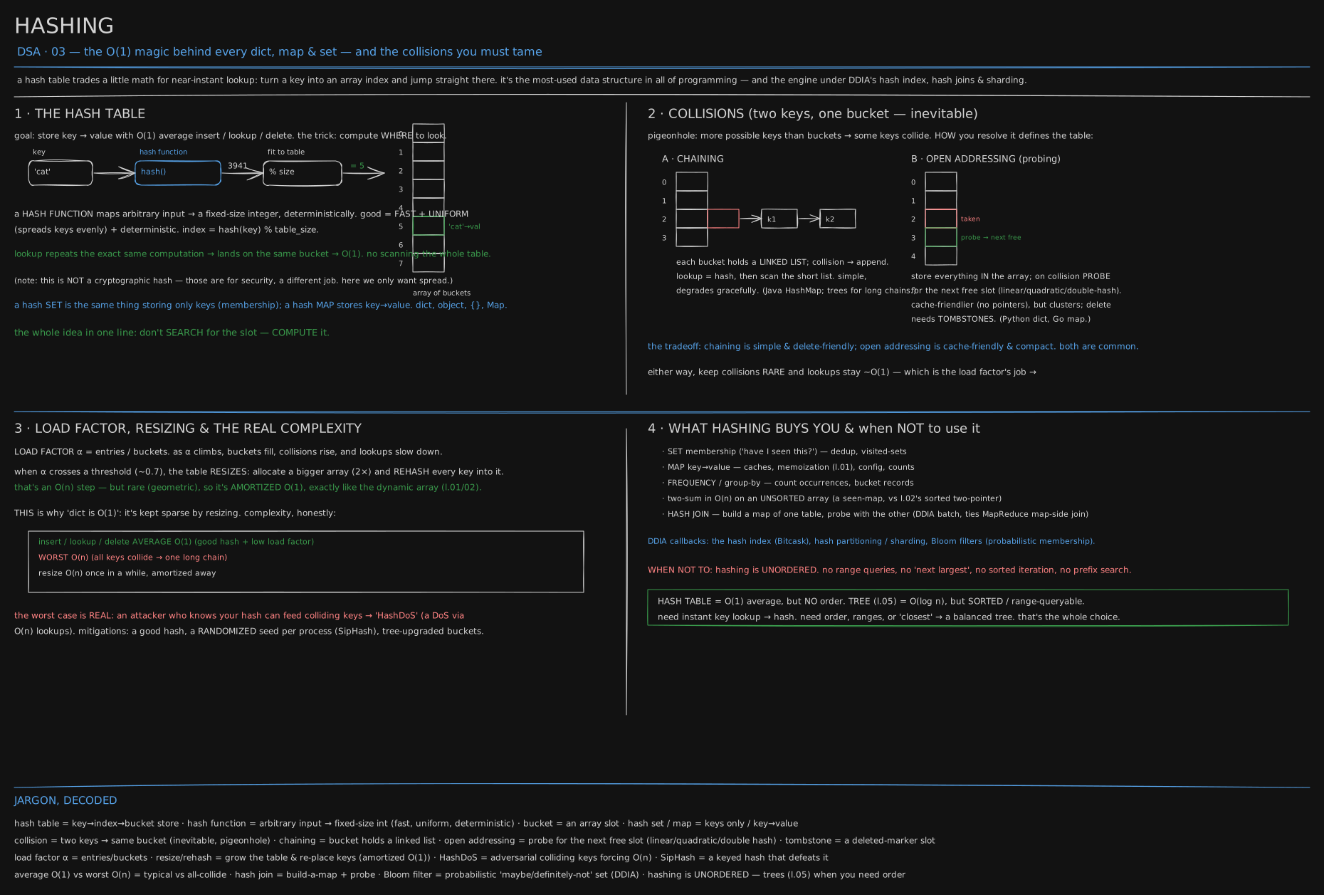
Here it is on a word you already know. Take ‘cat’ and run it through a fixed recipe of arithmetic on its letters. The exact recipe doesn’t matter here; say it gives 3941. A wall of 8 boxes can’t use 3941 directly, so take the remainder after dividing by 8. Eight 492s make 3936, and 3941 − 3936 leaves 5. ‘cat’ lands in box 5, and it lands there every time, on any wall of 8 boxes, forever.

flowchart LR
  K["key: 'cat'"] -->|"one small sum"| N["3941"]
  N -->|"remainder after ÷ 8 boxes"| B["box 5"]

Notice something else: a box doesn’t just hold the answer, it holds the question too - the key sits right beside its value. That’s the only way a box can tell ‘cat’ apart from any other word that happens to land there: it checks the key it actually stored, not just whatever value is sitting in the box.

You’ve already used this exact wall of boxes, built for you:

• Python’s dict
• JavaScript’s {} and Map
• Go’s map
• Java’s HashMap

Two letters, one box

A wall of 8 boxes and a country full of possible words cannot give every word its own box. Sooner or later two different keys compute to the same number - ‘cat’ might share box 5 with a thousand other words that also land there. That clash is a collision, and it isn’t a bug: with more possible keys than boxes, it’s guaranteed by simple counting. Put more letters than boxes into a wall and some box must hold two.

So a box needs a rule for holding more than one letter. Some post offices let a box hold a small stack, in the order the letters arrived - engineers call each box on the wall a bucket, and a bucket that holds a stack resolves a collision by writing the new letter underneath the old one. Fetching ‘cat’ back means landing on box 5, then reading down the stack until a letter says ‘cat’ back to you.

flowchart TD
  A["fetch 'cat', compute box 5"] --> B{"box 5 empty?"}
  B -- yes --> C["not here"]
  B -- no --> D["read the top letter in box 5"]
  D --> E{"is it 'cat'?"}
  E -- yes --> F["found it"]
  E -- no --> G{"another letter under it?"}
  G -- yes --> D
  G -- no --> C

Other post offices do it differently: if box 5 is taken, the letter goes in box 6 instead, and a search that lands on a full box just keeps checking the next one along. Both ways work. Both still get you to the right neighbourhood in one sum, even when that exact box is busy.

How full is too full

A wall that’s nearly empty almost never collides. A wall that’s nearly full collides constantly, and every collision means one more letter to read down a stack, or one more box to check along the row. How full a wall is has a name: the load factor - how many letters are on the wall, divided by how many boxes it has.

Post offices don’t wait until the wall is completely full. Once it passes about seven-tenths full, the whole wall gets a resize: a new, bigger wall goes up, and every single letter gets moved across, computed fresh for its new box. That’s slow, once, for every letter on the wall - but it happens rarely, and it happens before the wall gets bad enough to matter, so spread across every letter ever posted it costs almost nothing per letter.

There is one more twist, saved for the second read: what happens when someone works out your sum on purpose, and points every key at the same box.

You now know

• A hash table finds a key by computing its box, not by searching for one.
• That computation is a hash: same key in, same box out, every time.
• Two keys landing on the same box is a collision, guaranteed once there are more keys than boxes.
• A box (bucket) that holds more than one key needs a rule for reading them back: a stack, or the next box over.
• How full the wall is has a name, the load factor, and past about 0.7 full the whole wall resizes.
• Computing the box costs the same no matter how many keys you store - until someone works out your sum on purpose.

Stop here if you want. What follows is the same wall of boxes in numbers, for when you want to see it turn.

Second read: the wall of boxes, in numbers

Formally: index = hash(key) % table_size. A hash function maps an arbitrary key to a number; %, the remainder after division, is what fits any size of hash number into a table of any size.

'cat' → hash() → 3941 → % 8 → index 5 → buckets[5] = value

A hash set stores keys only, for membership; a hash map stores key→value. A good hash is fast, uniform, and deterministic - and it is not a cryptographic hash, which solves a different problem, security rather than spread (Cryptography Foundations).

Chaining vs open addressing. The stack-in-a-box from the story is chaining: each bucket holds a linked list, and a collision appends to it - simple, handles deletion and high load gracefully (Java’s HashMap chains, and upgrades a long chain to a balanced tree). The next-box-over from the story is open addressing: every entry lives in the array itself, and a collision probes for the next free slot - linear, quadratic, or double hashing - with lookups following the same sequence (Python dict, Go map). Open addressing is cache-friendlier (the next slot to check sits right beside the last one in memory) and more compact, but it clusters as it fills, and deleting a key needs a tombstone - a “was-here” marker, so a probe sequence doesn’t break early.

Load factor, formally. α = entries / buckets. Past roughly 0.7, the table resizes: it allocates a bigger array, typically 2×, and rehashes every key into it - an O(n) step, but rare, so spread across every cheap insert that came before it, it’s amortized O(1):

insert / lookup / delete   average O(1)   (good hash + low load factor)
                           worst   O(n)   (all keys collide → one long chain)
                           resize  O(n)   occasionally, amortized away

Where 1 + α/2 comes from. With n keys spread over m buckets, the average bucket holds n/m = α keys - that’s what the load factor is. A successful lookup lands in its own key’s bucket and scans on average halfway down it, α/2 other keys, plus the one comparison that finds it: 1 + α/2. At α = 0.7 that’s 1.35; the measured 1.32 below is that formula with a real hash instead of a perfect one. The last column, (1 + 1/(1−α)²)/2, is the textbook estimate for open addressing on a lookup that misses (a key that is not there, so the probe runs to an empty slot); it is not the same quantity as the measured average beside it, but it shows the shape. It climbs far faster, because a run of occupied slots makes every later key more likely to land in it and extend the run further - clusters feed themselves.

Measured on 65,536 buckets, a decent string hash (FNV-1a), Node v22.22.3:

alpha   chaining avg  longest chain   linear-probe avg  longest probe   1+alpha/2   (1+1/(1-a)^2)/2
0.25            1.12              4              1.17              6       1.13             1.39
0.50            1.24              4              1.49             18       1.25             2.50
0.70            1.32              5              2.02             52       1.35             6.06
0.90            1.42              6              4.74           1730       1.45            50.50
0.95            1.45              6             36.99          10523       1.48           200.50
0.99            1.47              7            320.47          39315       1.50          5000.50
2.00            1.96              9         (open addressing cannot exceed 1.00)
4.00            2.98             14         (open addressing cannot exceed 1.00)

Two rows carry the point. At 0.7 both structures are cheap: 1.32 vs 2.02 probes. At 0.9 chaining has moved to only 1.42 while linear probing’s longest probe has gone from 52 to 1,730 - that gap is the entire argument for resizing before 0.9. Chaining degrades gently even past 1.0 (average 2.98 at α = 4, longest chain 14); open addressing simply cannot exceed α = 1, and the cliff just before it is why CPython resizes at two-thirds full while Java’s HashMap can afford to wait until 0.75.

The worst case, measured. If every key is made to collide - eight buckets, a hash that returns 0 for everyone - each insert has to scan the whole bucket for a duplicate before appending, against a normal Map doing the same inserts:

n       all-collide ms   good-hash ms
1000                3.1          0.05
2000                8.8          0.17
4000               28.3          0.46
8000              100.9          0.54
16000             296.6          0.81

Doubling n roughly triples-to-quadruples the all-collide time - the O(n²) signature: every insert walks the whole chain so far, so n inserts cost about n²/2 comparisons (at n = 16,000 that’s 128 million comparisons, and 296 ms over 1.28 × 10⁸ is about 2.3 ns each, one string compare per couple of clock ticks). The good-hash column stays roughly linear. At n = 16,000 the gap is already 366×; at the million-row size a real request body can carry, the quadratic version would run for hours. That gap is HashDoS: an attacker who works out which keys collide can freeze a server with ordinary-looking input, the same class of attack The bouncer at the door (rate limiting) rate-limits away. The fix is a hash seeded randomly per process - SipHash is one built for exactly this - so nobody outside the process can predict which keys will collide in it. Run python3 -c 'print(hash("cat"))' twice and you’ll get two different large numbers; pin the seed with PYTHONHASHSEED=0 and both runs agree.

O(1) is flat, and the resize is visible. A lookup’s cost shouldn’t depend on n. Measured on a Map of string keys, one million lookups at each size:

n        build ms   lookup ns/op
1000          0.1           11
10000         1.2           13
100000       12.4           12
1000000     279.8           17

A thousand times more data, 11 ns to 17 ns. The small climb at a million is the CPU cache running out, not the algorithm: the table no longer fits in fast memory, so some lookups pay for a trip to RAM.

CPython’s dict reports its own byte size, and it only changes when the table is rebuilt:

entries  bytes
0        64
1        224
6        352
11       632
22       1168
43       2264
86       4688
171      9304

Each jump is roughly the previous one doubled, geometric growth, and fires when the table is about two-thirds full. Between jumps an insert costs nothing extra; on a jump every existing key gets rehashed.

Classic pitfalls.

• A key that can change is not a key. Python refuses outright: with lst = [1, 2], the line d[lst] = 1 raises TypeError: unhashable type: 'list'; use a tuple (1, 2) instead.
• Hash and equality must agree. Two keys that compare equal must hash equal, or a lookup computes one slot while the stored copy sits in another.
• Plain JS objects turn every key into a string: o[1] = 'num'; o['1'] = 'str' leaves one key holding 'str', not two. A Map keeps 1 and '1' apart; reach for Map whenever keys aren’t known-safe strings.
• NaN isn’t equal to itself, but Map special-cases it so m.set(NaN, 'x'); m.get(NaN) still works; 0.1 + 0.2 !== 0.3, so computed floats make unreliable keys too.
• Iteration order isn’t sort order. JS Map and Python 3.7+ dict iterate in insertion order; Go deliberately randomises it so nobody can depend on it.
• None of this protects you if untrusted input becomes keys and you’ve replaced the runtime’s seeded hash with a “faster” one of your own.

What this buys you, and when not to reach for it. Set membership (seen-before checks, dedup), map key→value (caches, memoization, Complexity & Big-O), frequency and group-by counts, two-sum on an unsorted array in O(n) via a seen-map (versus Arrays & Strings‘s sorted two-pointer, O(n) time and O(1) space but a sort first), and a hash join - build a map of one table, probe with the other, the way batch processing does it (Batch Processing). The same idea underlies Bitcask’s hash index and hash partitioning; Bloom filters push it further, a small array of bits that can say “definitely not here” for certain, using several hashes over the same key.

What it costs: a hash table is unordered. No range queries, no “next largest”, no sorted iteration, no prefix search. Need instant lookup by exact key: hash. Need order, ranges, or “closest”: a tree.

Try it

# collisions and worst case, made visible
class BadHash:
    def __hash__(self): return 1          # everything lands in one bucket
    def __eq__(self, o): return self is o
d = {}
import time
xs = [BadHash() for _ in range(20_000)]
t=time.perf_counter()
for x in xs: d[x] = 1                      # O(n) per insert → O(n^2) total: slow
print("adversarial", time.perf_counter()-t)

# the everyday power: frequency + dedup + O(n) two-sum
from collections import Counter
print(Counter("mississippi"))             # char frequencies in O(n)
def two_sum(a, t):
    seen = {}
    for i, x in enumerate(a):
        if t - x in seen: return (seen[t-x], i)
        seen[x] = i
print(two_sum([2,7,11,15], 9))            # (0, 1) - unsorted, O(n)

Three more, each under a minute. They produce the numbers quoted above, so run them and compare.

# 1. the per-process seed: two different numbers, then the same number twice
python3 -c 'print(hash("cat"))'; python3 -c 'print(hash("cat"))'
PYTHONHASHSEED=0 python3 -c 'print(hash("cat"))'; PYTHONHASHSEED=0 python3 -c 'print(hash("cat"))'

# 2. watch the resizes: the byte size only changes when the table is rebuilt
python3 -c '
import sys
d = {}; last = sys.getsizeof(d); print(0, last)
for i in range(1, 200):
    d[i] = i; s = sys.getsizeof(d)
    if s != last: print(i, s); last = s'

# 3. object keys vs Map keys in JS: one key or two?
node -e 'const o={}; o[1]="num"; o["1"]="str"; console.log(Object.keys(o).length, o[1]);
         const m=new Map(); m.set(1,"num"); m.set("1","str"); console.log(m.size, m.get(1), m.get("1"))'

Expected: run 1 prints two different large integers, then 692052486964499043 twice. Run 2 prints the jump table from the resize section. Run 3 prints 1 str and then 2 num str.

And the load-factor experiment, if you want to reproduce the probe table (change m or the α list and re-run; it takes a few seconds):

// probes.mjs - chaining vs linear probing, probes per successful lookup
function fnv(s){ let h = 0x811c9dc5; for (let i=0;i<s.length;i++){ h ^= s.charCodeAt(i); h = Math.imul(h, 0x01000193); } return h >>> 0; }
function chaining(n, m) {
  const b = Array.from({length: m}, () => []);
  for (let i=0;i<n;i++) b[fnv('k'+i) % m].push('k'+i);
  let probes = 0, longest = 0;
  for (let i=0;i<n;i++){ const c = b[fnv('k'+i) % m]; longest = Math.max(longest, c.length); probes += c.indexOf('k'+i) + 1; }
  return { avg: probes / n, longest };
}
function linear(n, m) {
  const t = new Array(m).fill(null);
  for (let i=0;i<n;i++){ let j = fnv('k'+i) % m; while (t[j] !== null) j = (j+1) % m; t[j] = 'k'+i; }
  let probes = 0, longest = 0;
  for (let i=0;i<n;i++){ let j = fnv('k'+i) % m, p = 1; while (t[j] !== 'k'+i){ j=(j+1)%m; p++; } probes += p; longest = Math.max(longest, p); }
  return { avg: probes / n, longest };
}
const m = 1 << 16;
for (const a of [0.25, 0.5, 0.7, 0.9, 0.95, 0.99]) {
  const n = Math.round(a * m), c = chaining(n, m), l = linear(n, m);
  console.log(a, 'chain', c.avg.toFixed(2), c.longest, 'linear', l.avg.toFixed(2), l.longest);
}

Go deeper

• Python dict internals (open addressing, compact dict) + Raymond Hettinger - “Modern Dictionaries” (talk)
• Java 8 HashMap: chaining + treeify
• SipHash & HashDoS
• CLRS ch. 11 (hash tables)
• Robin Hood hashing.

Related

• Foundations #04 - Hashing (O(1) "yaad") - the Hinglish twin of this lesson, with its own measured tables (naive vs djb2 hash, Map vs {}) and the three interview patterns; its board has a lab, O(1) yaad, where a fixed list of 276 keys goes through a bad hash and a good one and you watch the deepest chain and the probe count at 99% full.
• Clinic #05 - Two Sum - the “seen map” pattern from this lesson, as a full worked problem.
• Clinic #06 - Longest Substring Without Repeating Characters - a hash map of last-seen positions driving a sliding window.
• Clinic #20 - Top K Frequent Elements - frequency counting, then bucketing by count.
• Linked Lists, Stacks & Queues - the linked list each chaining bucket is made of.
• Trees (BST, balancing, heaps, tries) - the ordered alternative when you need ranges or “next largest”.
• Redis: The Map (SET / GET / DEL) in From Scratch builds this for real: Redis’s own table, chaining and the incremental resize, in Go.
• The full DSA list is in CURRICULUM.

Retrieval practice

9 questions. Answer each one before you open it.