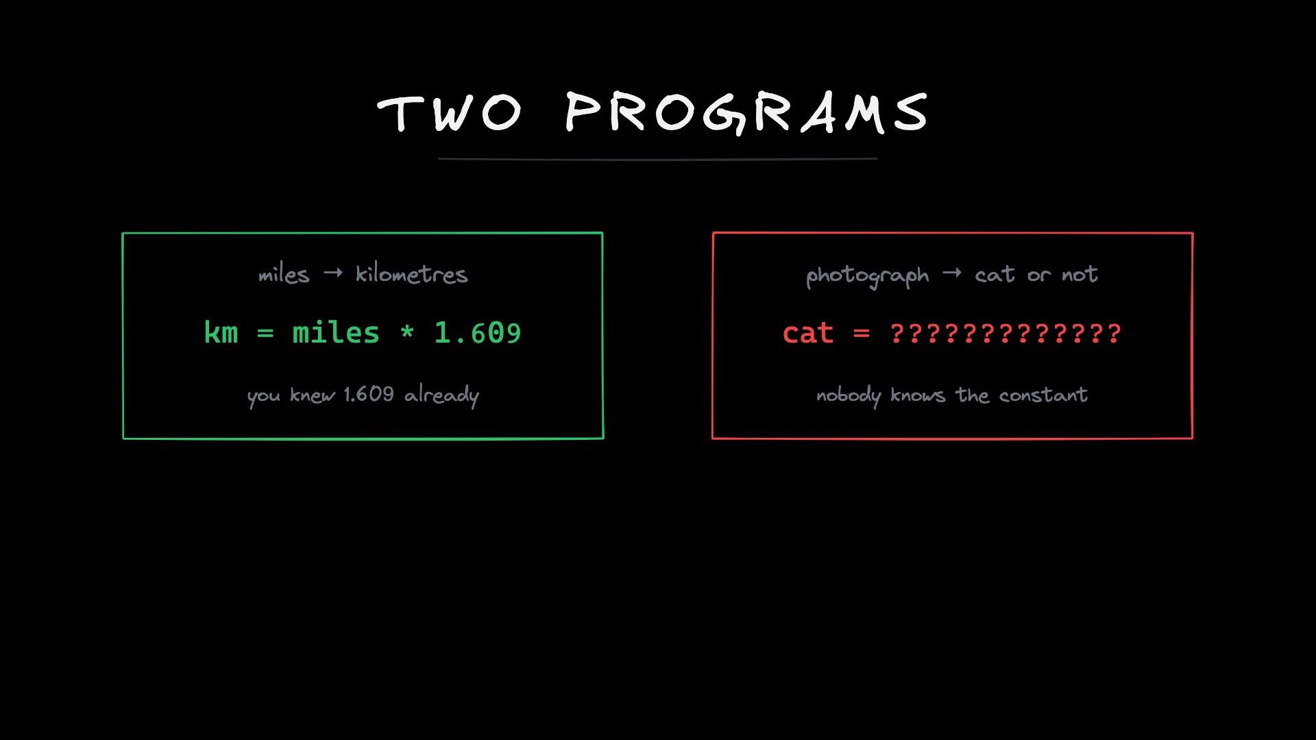
How It Learns (loss, gradient descent, backprop)
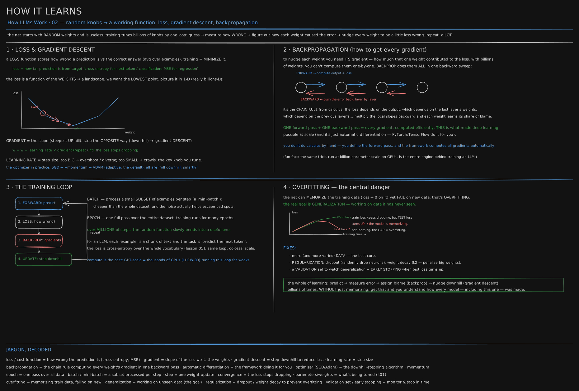
The How It Learns board, in the How LLMs Work track. The last lesson built a machine out of dials and set nine by hand. This is how a machine came to turn its own, including the middle ones, which took the field seventeen years to work out.
Before you start. You need What a Neural Network Is, which gave you this: a network is rows of small units, each adding up weighted votes and passing the total on, with one rule between the rows that turns negative totals into zero. Everything the machine knows sits in those dials, formally called weights, and that lesson ended by admitting nobody knew how to turn the middle ones.
Assigning blame: which middle dial made the answer wrong
Rosenblatt’s 1958 machine turned its own dials by a rule that fits in a sentence. Show it a shape, it answers, and if the answer is wrong, every dial that pushed the answer the wrong way gets turned a little the other way. That works because every dial in his machine feeds the answer directly. You can see what each one did.
Now put a row of units in the middle, the fix that solved the two-switch door in the last lesson (the door that opens when exactly one of two switches is on, which no single unit could learn). A middle dial does not touch the answer. It feeds a middle unit, which feeds another dial, which feeds the answer. The answer comes out wrong. How much of that was this dial’s fault? Up or down, and by how much? The name for that problem fits it: assigning blame. Hold on to the word. It is the only idea in this lesson.
Nudging one dial at a time: the obvious method, and the six and a half years it costs
There is an obvious way to find out what a dial is worth. Nudge it, run the network again, see whether the wrongness went down or up. For nine dials this is fine: run it ten times instead of once and you know everything.
Now count it for a real model. One pass through 175 billion dials costs about two operations per dial, so 350 billion, and nudging every dial once means one pass per dial: around 6 × 10²² operations. A 2020-era graphics card manages roughly 300 trillion useful operations a second, so that is six and a half years, for one step, on one example, of a loop needing millions of steps. The loop everyone could describe in a sentence was the loop nobody could run.
The loss: wrongness as one number you can watch fall
Before anything can go downhill, wrongness has to become a single number. Five points on a line: when x is 0, 1, 2, 3, 4 the right answer is 1, 3, 5, 7, 9. The machine is two dials, answer = w × x + b, both at zero, so every answer is 0 and the misses are 1, 3, 5, 7, 9. Square each and average:
(1 + 9 + 25 + 49 + 81) / 5 = 33Squaring does two jobs. Over-guessing and under-guessing both count as wrong, and a miss of 9 counts eighty-one times worse than a miss of 1, so big misses dominate. One number. Thirty-three. It is called the loss, and training means one thing: make it smaller.
Gradient descent: walking downhill, and the learning rate that sets the step
The loss is a number you get after you set the dials, so picture a landscape: every setting is a spot on the ground and the height there is the loss. Training is walking downhill.
At each spot you want one thing per dial. Raise it slightly: does the loss go up or down, and how fast? That is the dial’s slope. Collect one per dial and together they point straight uphill, so walk the other way:
new dial = old dial − step size × slopeIn English: if raising a dial raises the loss, lower it, in proportion to how much it mattered. That is gradient descent. Here the slopes are −14 and −5, so the loss falls if either dial rises and gradient descent raises both.
The only free choice left is how far to step, called the learning rate. Same points, same slopes, only the learning rate (the step size) changed:
| learning rate | loss at step 10 | what happened |
|---|---|---|
| 0.05 | 0.03 | found it |
| 0.5 | 875,882,809 | flew apart |
| 0.001 | 28.9 | barely moved |
At a learning rate of 0.05 the dials settle on 2.005 and 0.987. At 0.5 the first step throws the slope dial from 0 to 7, past the answer of 2, the next overcorrects to −9.5, and every step after lands further out on the other side. At 0.001 nothing goes wrong and nothing gets done.
flowchart LR
  F["forward: guess"] --> L["loss: 33"]
  L --> G["a slope for every dial"]
  G -->|"−14 and −5"| U["turn each dial against its slope"]
  U -->|repeat| F
Every training run in this track is those four boxes, and the loop they make is gradient descent. I wrote the third one by hand because there were two dials. That box is the six-and-a-half-year one.
9 October 1986: backpropagation, the blame flowing backwards
The answer had already been written down. In 1974 a Harvard doctoral student named Paul Werbos submitted a thesis called Beyond Regression with the method spelled out in it. The field did not pick it up, and through the winter the same idea was found and lost more than once by people who did not know about each other.
The version that stuck was four pages in Nature, by David Rumelhart and Ronald Williams at UC San Diego and Geoffrey Hinton, then at Carnegie Mellon. The title is the whole idea: “Learning representations by back-propagating errors.” A learning procedure, they write, “must decide under what circumstances the hidden units should be active.”
The trick is bookkeeping, not new mathematics. Run the network forward once, keep every intermediate total, then walk back from the answer. At the output you know the miss exactly, because that is what you measured. Hand it backwards along each connection, multiplying by the dial it crosses. Every middle unit now holds a number: its share of the blame. And once a unit knows its blame, every dial feeding it gets a slope by one multiplication:
slope of a dial = blame arriving from above × the input that dial multipliesIn English: a dial is answerable in proportion to how much blame reached it, and how loud the thing it was listening to was. Here it is on one unit. Input 2, dial 0.5, the bar (the bias, the amount added before the total is read) set to zero, right answer 3.
flowchart LR
  X["input = 2"] -->|"dial 0.5"| Z["total = 1"]
  Z --> Y["passes through: 1"]
  Y --> L["target 3, loss = 4"]
  L -.->|"blame at the answer: −4"| Y
  Y -.->|"rule's slope is 1, so −4 passes"| Z
  Z -.->|"× input 2"| S["slope for the dial: −8"]
Solid arrows go forward, dotted arrows carry blame back. One turn at a learning rate of 0.1 moves the dial to 1.3, the answer becomes exactly 3, the loss is zero.
Now notice what makes it cheap. That −4 was computed once and reused by every dial behind this unit; a million dials behind it would reuse the same −4. One pass forward, one pass back, and every slope in the network falls out at once, for about three times a forward pass, at any model size. That is backpropagation.
Back to the 175 billion dials. Nudging and retesting needed 6 × 10²² operations for one step, or six and a half years. Backpropagation needs about 10¹²: three and a half milliseconds on the same card.
Colin has two aunts: learning representations, what the middle rows build on their own
The paper still had to show this bought something a hand-built machine could not. So they gave a network two family trees of the same shape, one English and one Italian: twenty-four people, and twelve relationships, father, mother, husband, wife, son, daughter, uncle, aunt, brother, sister, nephew, niece. Every fact is a triple, person and relationship and person. They trained on 100 of the 104 and held four back.
Ask it Colin, has-aunt. It lights two answers, because Colin has two aunts. Nobody told it to look for aunts.
Then they looked at what the middle rows had made of themselves. One unit had become a detector for English versus Italian, another encoded generation, another which branch of the family. Nobody asked for any of those. They are what you have to notice to answer questions about families, and the loop found them because noticing them lowered the loss.
That is what “learning representations” means. Middle dials do not merely take good values. They arrange themselves into a description of the problem. Every feature a language model has, grammar and tense and tone and the difference between a question and an order, arrived this way. Nobody wrote it. Backpropagation built it.
Overfitting: the training loss falls while the machine gets worse
The loop has a failure that does not look like failure, so you have to go looking for it. Take six points sitting roughly on a line, with a little measurement noise. Fit a straight line, two dials: its loss on those six points is 0.048. Now fit a bendy curve with six dials, one per point, so it passes through every one exactly. Its loss is 0.000. Perfect score.
Score both on fifty fresh points from the same rule, which neither fit has seen. The line gets 0.079. The curve gets 0.174, more than twice as wrong, because between the six points it bent to chase noise, and noise does not repeat.
Watch only the training loss and you pick the worse model every time, the number on your screen falling while the machine gets worse. That is overfitting, and it is why you hold data back: the only honest number is measured on examples the dials never touched. Every cure takes away the room to memorise. Give that curve sixty training points and its held-out score drops to 0.071, next to the line’s 0.069.
You now know
- Training is one loop: guess, measure the loss, work out each dial’s share of the blame, turn every dial the other way, repeat.
- The loss is wrongness boiled down to a single number, and training only ever makes the loss smaller.
- Each dial has a slope. Walking against those slopes is gradient descent, and the learning rate alone decides between arriving, flying apart and crawling.
- Finding the slopes by nudging one dial at a time is hopeless at scale: six and a half years for one step of a large model.
- Backpropagation gets all of them in one backward sweep, for about three forward passes, by handing the miss backwards and multiplying as it goes.
- A loop that drives the training loss to zero may be overfitting, memorising the examples instead of learning the rule. Only a score on data it never touched tells you which.
Stop here if you want. What follows is the same loop in numbers, for when you want to watch it turn.
Second read: the same loop in numbers
The line, three step sizes, 200 steps. Loss is the average of (pred − y)², called mean squared error. The slopes are dL/dw, the average of (pred − y) × x, and dL/db, the average of (pred − y); the factor of 2 from differentiating the square is dropped, since it only rescales the step.
--- lr=0.05
step   0  w=   0.000 b=   0.000 loss=     33.0000
step   1  w=   0.700 b=   0.250 loss=     14.6025
step  10  w=   2.045 b=   0.759 loss=      0.0269
step 199  w=   2.005 b=   0.987 loss=      0.0001
--- lr=0.5
step   1  w=   7.000 b=   2.500 loss=    182.2500
step   2  w=  -9.500 b=  -3.250 loss=   1007.0625
step  10  w=-10785.857 b=-3783.235 loss=875882809.4181
--- lr=0.001
step  10  w=   0.136 b=   0.049 loss=     28.8504
step 199  w=   1.539 b=   0.557 loss=      2.2906
w arrives first and b crawls in last, because the slope dial’s gradient is multiplied by x, which runs up to 4. That uneven speed is what Adam and its per-dial step sizes are for; the progression is gradient descent, then momentum, then Adam.
The backward walk, named properly. It is the chain rule, every factor on one ReLU unit:
x, w, b, target = 2.0, 0.5, 0.0, 3.0
z = w*x + b; y = max(0.0, z); loss = (y - target)**2
dL_dy = 2*(y - target); dy_dz = 1.0 if z > 0 else 0.0
dL_dw = dL_dy*dy_dz*x;  dL_db = dL_dy*dy_dz*1.0
print("y", y, "loss", loss, "dL/dy", dL_dy, "dL/dw", dL_dw, "dL/db", dL_db)
w, b = w - 0.1*dL_dw, b - 0.1*dL_db
y = max(0.0, w*x + b); print("after one step: w", w, "b", b, "y", y, "loss", (y-target)**2)
y 1.0 loss 4.0 dL/dy -4.0 dL/dw -8.0 dL/db -4.0
after one step: w 1.3 b 0.4 y 3.0 loss 0.0Two things fall out. Had z been negative, dy_dz would be 0 and nothing behind the unit would receive any blame, the dead neuron problem in one line. And the × x on every slope is why inputs are normalised first: a feature ranging to 1000 hands its dials gradients a thousand times everyone else’s. You never write this by hand; the framework walks your forward pass backwards, which is automatic differentiation.
Two words for the outer loop. A batch is a subset of examples used for one update, noisy in a way that helps escape bad spots; an epoch is one full pass over the data. For a language model each example is a span of text, the task is the next token, and the loss is cross-entropy over the vocabulary (From Transformer to LLM).
“Weeks” is arithmetic. Each training token costs about 6 × parameters operations, 2 forward and 4 backward, since the chain rule needs the dial’s slope and the blame to pass back.
 FLOPs           6 × 175 B params × 300 B tokens        = 3.15 × 10²³
 one GPU         ~3 × 10¹⁴ FLOP/s useful (a 2020 A100 at ~30% utilisation)
 one GPU alone   3.15 × 10²³ ÷ 3 × 10¹⁴  = 10⁹ s       ≈ 33 years
 1,000 GPUs      33 years ÷ 1,000                       ≈ 12 days   ✓ "weeks"
Double both and the bill quadruples, which is why a model’s size and its data are always quoted together.
Overfitting, measured, with no network at all, because overfitting is a property of fitting. Six noisy training points on y = 2x + 1, noise of standard deviation 0.3 so the floor is about 0.3² = 0.09, and 50 held-out points.
import numpy as np
rng = np.random.default_rng(1)
xs = np.linspace(-1,1,6);  ys = 2*xs + 1 + rng.normal(0,0.3,6)    # 6 training points
xt = np.linspace(-1,1,50); yt = 2*xt + 1 + rng.normal(0,0.3,50)   # 50 held-out
for deg in (1,2,5):
    c = np.polyfit(xs, ys, deg)
    tr = ((np.polyval(c,xs)-ys)**2).mean(); te = ((np.polyval(c,xt)-yt)**2).mean()
    print(f"degree {deg} ({deg+1} knobs): train MSE {tr:.3f}   test MSE {te:.3f}")
degree 1 (2 knobs): train MSE 0.048 test MSE 0.079
degree 2 (3 knobs): train MSE 0.041 test MSE 0.077
degree 5 (6 knobs): train MSE 0.000 test MSE 0.174The named cures map onto this table. More data: sixty points instead of six and the degree-5 fit scores 0.071 held out, against the line’s 0.069. Weight decay penalises large coefficients, so the curve cannot bend hard. Dropout randomly silences units while training. Early stopping catches the network at the straight-line answer, which it reaches first. A validation set lets you see any of it.
Try it
import numpy as np
# fit y = 2x + 1 by gradient descent on MSE - learning in six lines
xs = np.array([0,1,2,3,4.]); ys = 2*xs + 1
w, b, lr = 0.0, 0.0, 0.05
for step in range(200):
    pred = w*xs + b
    err  = pred - ys                          # dLoss/dpred
    gw   = (err*xs).mean(); gb = err.mean()   # the two slopes, by hand
    w -= lr*gw; b -= lr*gb                    # gradient-descent step
print(round(w,2), round(b,2))                 # 2.0  0.99 - it found the function
Bump lr to 0.5 and watch it diverge; drop it to 0.001 and watch it crawl. That block printed the table above.
Take the chain-rule block and set w = -0.5. z goes negative, dy_dz becomes 0, and both slopes print -0.0. The neuron is dead for this example and no step size revives it.
Then take the overfitting block and change both 6s in the first linspace call to 60. Held-out error for the six-dial fit falls from 0.174 to 0.071. More data is the best cure because it is the only one that removes the room to memorise.
Go deeper
- Rumelhart, Hinton & Williams (1986), the four pages themselves
- 3Blue1Brown - Gradient descent & Backpropagation
- Andrej Karpathy - the spelled-out intro to backpropagation
- Michael Nielsen - how backprop works (ch. 2)
- Distill - Why Momentum Really Works.
Related
- What a Neural Network Is is the machine whose dials this lesson turns; the
× xon every slope is that lesson’s forward pass read backwards. - From Transformer to LLM is this loop at full scale: cross-entropy over a vocabulary, trillions of tokens.
- Fine-tuning & Alignment runs it again on an already-trained model, with a different loss.
Retrieval practice
10 questions. Answer each one before you open it.
What question did the last lesson leave open, and what is the name for it?
Rosenblatt turned dials by looking at the answer: wrong answer, turn the dials that caused it. That works only because every dial feeds the answer directly. A middle dial feeds a middle unit, which feeds another dial, which feeds the answer, so there is no obvious way to say how much of the error was its fault. That is assigning blame, unsolved at useful scale from 1969 to 1986.
Why can you not just nudge each dial and re-run the network to see what it was worth?
It costs one forward pass per dial. For 175 billion dials one pass is about 350 billion operations, so nudging every dial once is roughly 6 × 10²² operations: six and a half years on a card doing 300 trillion useful operations a second, for one step on one example. Backpropagation does it in three and a half milliseconds.
What is a loss function, why is the miss squared, and what does training do to it?
The loss turns wrongness into one number you can watch fall: square every miss and average, which is mean squared error. Squaring makes over-guessing and under-guessing both count as wrong, and makes big misses dominate, since a miss of 9 scores eighty-one times a miss of 1. Language models use cross-entropy instead, but the role is identical.
Explain gradient descent and the role of the learning rate.
Every setting of the dials is a spot on a landscape whose height is the loss. Each dial has a slope, how fast the loss rises if you raise it, and together they point uphill, so you move the other way: new dial = old dial − step size × slope. The step size is the learning rate: too large overshoots, too small crawls. Adam sets it per dial.
Fitting y = 2x + 1 from five points with both dials at zero, the loss starts at 33. Where does that come from, and which way does the first update move the dials?
Every prediction is 0 against targets 1, 3, 5, 7, 9, so the loss is (1 + 9 + 25 + 49 + 81) / 5 = 33. Both slopes are negative, dL/dw = −14 and dL/db = −5, so the loss falls if the dials rise and the update raises both, to 0.7 and 0.25 at a learning rate of 0.05.
The same loop at a learning rate of 0.5 reached a loss of 875 million by step 10. Describe what each step did.
The first step threw w from 0 to 7, past the answer of 2. At 7 the slope points back the other way and is larger, so the next step overshot to −9.5, and every step after landed further from the bottom on the opposite side. That is divergence: the step is wider than the valley, so the loop climbs instead of descending.
What does backpropagation do on the backward walk, and why is it cheap?
It runs forward once keeping every intermediate total, then hands the miss backwards along each connection, multiplied by the dial it crosses. Every middle unit ends up holding its share of the blame, and each dial’s slope is then blame arriving from above × the input that dial multiplies. Each blame figure is computed once and reused by every dial behind it, so one pass forward and one back yields every slope.
One ReLU unit, x = 2, w = 0.5, b = 0, target 3. Compute the slope for w and say which factor would kill it if z were negative.
Forward: z = 1, y = 1, loss 4. Backward: dL/dy = 2(y − target) = −4, then dy/dz = 1 because z > 0, then dz/dw = x = 2. So dL/dw = −4 × 1 × 2 = −8. Had z been negative, dy/dz would be 0, every slope behind that unit would be 0, and nothing upstream would learn. That is the dead neuron problem.
The 1986 Nature network was given two family trees. What did it do that a hand-built machine could not, and what does “learning representations” mean?
Trained on 100 of 104 person-relationship-person triples across an English and an Italian tree, it answered held-out questions, lighting two answers for “Colin, has-aunt” because Colin has two aunts. Its middle units had organised themselves into detectors nobody asked for: English versus Italian, generation, branch of the family. Middle dials do not just take good values, they become a description of the problem.
Six noisy points: a six-dial curve scores a training loss of 0.000 while a straight line scores 0.048. Which is the better model, how do you know, and what is the curve’s failure called?
The line. Its 0.048 is about the noise floor, since noise of standard deviation 0.3 has variance 0.09, which is what an honest fit of noisy data should score. On 50 held-out points the line scores 0.079 and the curve 0.174, because the curve passed through the six points exactly and bends to chase noise between them. That is overfitting.