What a Neural Network Is
Opens the black box behind the assistant you talk to. This lesson tells the story of how that box was invented, killed, and brought back, and by the end of the story you will know what is inside it.
Before you start. You need to be able to multiply two numbers and add the results. That is the whole of the maths in the story half of this lesson. Everything else is people, a machine, and one table with four rows.
The problem nobody could code
In the 1950s a computer did exactly what you typed, and nothing else. If you wanted it to tell a 7 from a 1, you had to write the rules: a 7 has a flat stroke on top, then a slanted one down. Then someone writes a 7 with a bar through the middle. Then someone writes a lazy 7 that leans left. Then a 1 with a long flag at the top that looks like a 7. Every rule you add breaks on the next handwriting sample, and the rulebook grows without ever being finished.
Nobody could write that rulebook. Not because they were not clever enough, but because the rules do not exist in a form you can write down. You know a 7 when you see one, and you cannot say how.
A psychologist at Cornell named Frank Rosenblatt made a different bet. Do not write the rules. Build a machine that finds them itself, by being shown examples and told when it is wrong.
1958: the perceptron, a machine whose weights turn themselves
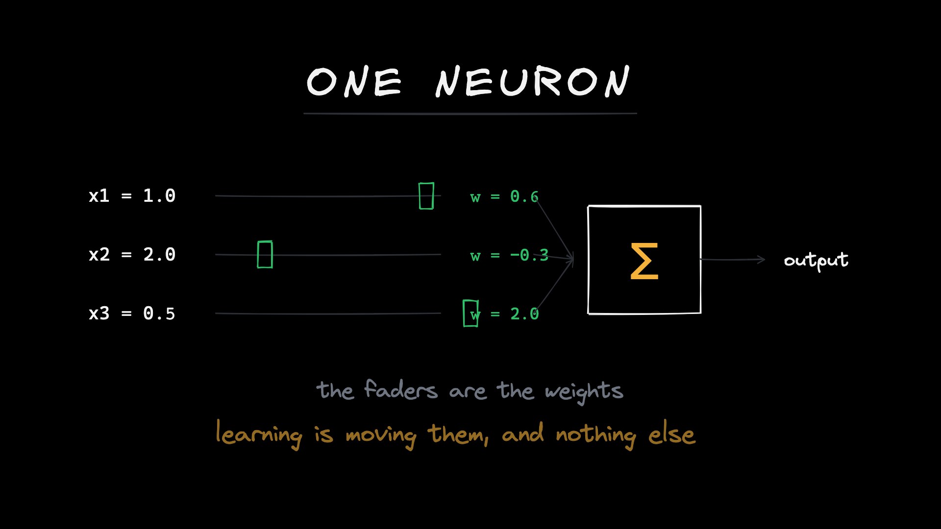
The Navy paid for it. It was called the Mark I Perceptron, and it filled a room. On the front was a camera of 400 light sensors in a 20 by 20 grid. Behind each sensor was a dial, a real one, a knob turned by a small motor. Show the camera a shape, and each sensor that sees light casts a vote. How much that vote counts is set by its dial. Add up all the votes. If the total clears a bar, the machine says “yes, that is the shape”. If it does not, “no”.
That is the entire machine. Sensors, dials, a sum, a bar. Here it is with two sensors instead of 400:
flowchart LR
  A["sensor A sees light: 1"] -->|"dial A: 0.8"| S["add the votes: 0.8 + 0 = 0.8"]
  B["sensor B dark: 0"] -->|"dial B: -0.3"| S
  S -->|"is 0.8 over the bar at 0.5?"| Y["yes"]
Sensor A is lit, so it votes 1, and its dial says that vote is worth 0.8. Sensor B is dark, votes 0, so its dial does not matter this time. Total 0.8. The bar is at 0.5. Over the bar: yes.
Now the part that made the newspapers. Nobody sets the dials. You show the machine a shape, it answers, and if it is wrong, every dial that contributed to the wrong answer gets turned a little the other way. Show it a thousand shapes and the dials settle somewhere that gives the right answer most of the time. The machine found the rules, and they are stored as 400 dial positions that no human ever wrote.
The New York Times, July 1958, quoting the Navy: the embryo of an electronic computer that will one day walk, talk, see, write, reproduce itself and be conscious of its existence. It was a lot to say about a machine that could tell left from right.
Three names, now that you have seen the things, and the rest of the lesson uses them:
- One sensors-dials-sum-bar unit is a neuron. The name is borrowed from the brain, but it is only arithmetic.
- A dial is a weight. A big weight means “this sensor matters a lot”, a weight near zero means “ignore this one”, a negative weight means “this sensor counts against”.
- The bar is the bias. Lower the bias and the neuron says yes more easily.
Rosenblatt’s machine, and any machine built from these, is a perceptron.
1969: XOR, the four-row table that killed it
Eleven years later, two MIT professors, Marvin Minsky and Seymour Papert, published a book called Perceptrons, and it ended the field for a generation. The blow was one small table.
Imagine a door with two switches. It opens when exactly one switch is flipped. Both off, closed. Both on, closed. One on, open. Four rows:
| switch A | switch B | door |
|---|---|---|
| off | off | closed |
| off | on | open |
| on | off | open |
| on | on | closed |
A child learns this rule in a minute. Engineers call it XOR, exclusive or: one or the other, not both. The perceptron cannot learn it at all, ever, with any weights. Here is why, and it is the one picture worth keeping from this lesson.
Draw the four rows as four dots on a square. “Both off” is the bottom left corner, “both on” is the top right, the two “one on” rows are the other two corners. The door is open on two corners that sit diagonally opposite each other, and closed on the other diagonal. Now try to draw one straight line that keeps the open corners on one side and the closed corners on the other. You cannot. Any line that separates the two open corners from each other fails, and any line that keeps them together sweeps in a closed corner too.
flowchart TB
  TL["off, on: OPEN"] --- TR["on, on: closed"]
  BL["off, off: closed"] --- BR["on, off: OPEN"]
  TL --- BL
  TR --- BR
A sum of weighted votes against a bias is exactly a straight line. Every setting of the weights is a different line, and no line does this. The machine that was going to be conscious could not learn a light switch. The Navy money stopped. Twenty years of what people now call the AI winter.
The fix: a hidden layer, and an activation that stays quiet
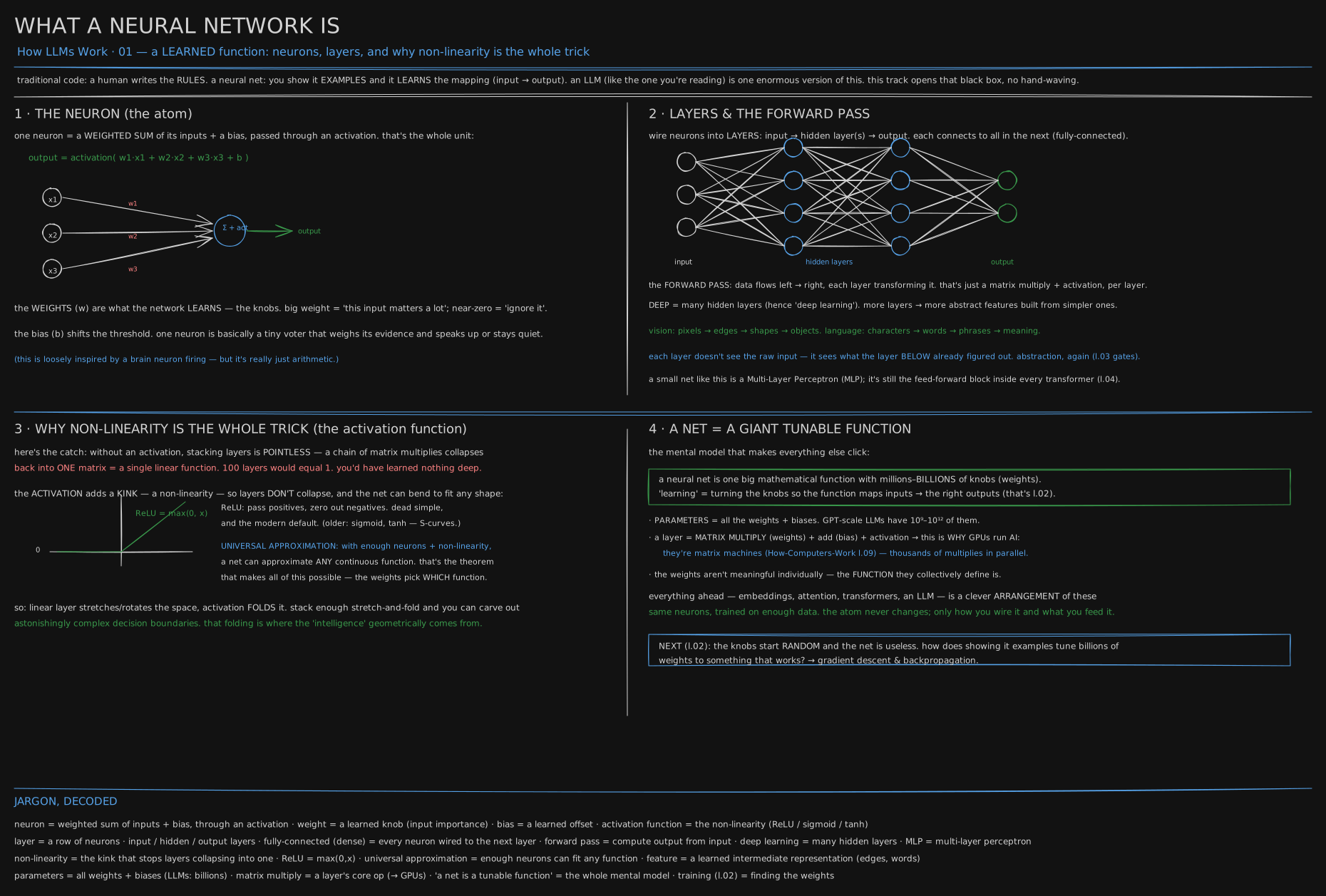
The way out was known even in 1969. Put a second row of neurons between the sensors and the answer. A row of neurons is a layer, and a layer that sits in the middle, touching neither the input nor the answer, is a hidden layer. Let the hidden layer look at the switches, and let the answer neuron look at the hidden layer instead of the switches directly.
There is a trap in that idea, and it matters. A layer of weights is “multiply and add”. Two layers of “multiply and add” is still “multiply and add”. If the first layer doubles everything and the second layer triples it, you have built a layer that six-times it, and one layer could have done that. Two layers of straight lines is one straight line. Stacking layers on its own buys nothing.
The trick is one rule sitting between the layers: if a neuron’s total comes out negative, it stays quiet and says zero. Positive totals pass through untouched. That is all. A neuron whose total is minus 2.5 does not pass minus 2.5 along, it passes 0. The rule is called the activation, and this particular one, “negative becomes zero”, is ReLU (rectified linear unit). The activation is the only step in the whole machine that is not multiply-and-add.
The activation breaks the straight line. Watch it solve XOR. Two hidden neurons, weights chosen by hand:
- Hidden neuron 1 adds the two switches. It counts how many are on: 0, 1 or 2.
- Hidden neuron 2 also adds the two switches, but its bias is set one higher, so its total is “how many are on, minus 1”. Then the activation: negative stays quiet. So it says 0 when no switch is on, 0 when one is on, and 1 only when both are on. It is a “both” detector, and it exists only because of the activation.
- The answer is hidden 1 minus twice hidden 2.
| switch A | switch B | hidden 1 counts | hidden 2 says “both”? | answer: 1 minus 2 × 2 | door |
|---|---|---|---|---|---|
| 0 | 0 | 0 | 0 | 0 | closed |
| 0 | 1 | 1 | 0 | 1 | open |
| 1 | 0 | 1 | 0 | 1 | open |
| 1 | 1 | 2 | 1 | 2 − 2 = 0 | closed |
Read the last row. Both on. Hidden 1 says 2. Hidden 2 wakes up and says 1. Two minus two is zero. Closed. Nine weights and biases, one activation, and the XOR that no straight line could learn is learned.
The activation is the step that makes the machine able to bend. Stack enough layers with an activation between each pair, and the thing can fit any shape at all. That is a proven theorem, but XOR already showed you why.
1986 and 2012: backpropagation, GPUs, and the thing you are talking to
If the fix was known in 1969, why the twenty-year winter? Because nobody knew how to turn the weights in the hidden layer. The perceptron turned its weights by looking at the answer: wrong answer, turn the weights that caused it. A hidden layer’s weights are not connected to the answer directly, so which way do you turn them? That question took until 1986 to answer properly. The answer is called backpropagation, and it is the next lesson, How It Learns (loss, gradient descent, backprop).
Then it needed to get big. In 2012 three researchers in Toronto trained a machine of this exact kind, layers of weights with an activation between them, on a million photos, using two gaming graphics cards, GPUs, because the multiply-and-add is exactly what those cards are built for. It beat every hand-written rulebook in the world at recognising what was in a picture, by a margin nobody had seen before. That was the moment the winter ended.
The assistant you are reading this on is the same machine, a neural network: layers of neurons with an activation between each pair. Many layers make it “deep”, which is all deep learning means. All of its weights and biases together are its parameters, and it has a few hundred billion of them instead of 400. It was shown most of the internet instead of a thousand shapes. The sensors are words instead of light, and there is one more idea between the layers that lets it look back at earlier words, which is lesson Attention & the Transformer. But the unit never changed: votes, weights, a sum, a bias, and an activation that stays quiet.
You now know
- A neural network is a machine that finds rules from examples, because the rules for “is this a 7” cannot be written by hand.
- One neuron is votes times weights, added up, against a bias. The weights are what it learns.
- One neuron is a straight line, and a straight line cannot learn XOR, the door with two switches.
- Stacking layers does nothing on its own, because two straight lines make a straight line.
- One activation between the layers, “negative stays quiet”, is what lets the machine bend. ReLU is why any of this works.
- Turning the hidden layer’s weights is the hard part. That is backpropagation, the next lesson.
Stop here if you want. What follows is the same machine in numbers, for when you want to see it turn.
Second read: the forward pass in numbers
Data flowing through the layers to an answer is the forward pass. Take the smallest network with a hidden layer: two inputs, two hidden neurons, one output. Every weight is chosen by hand, so nothing is learned yet. The inputs are x1 = 2 and x2 = -1. Hidden neuron 1 has weights 0.5 and 1.0 and a bias of 1.0. Hidden neuron 2 has weights -1.0 and 0.5 and a bias of 0. The output neuron reads the two hidden values with weights 1 and -2 and a bias of 0.5.
Hidden neuron 1: 2 × 0.5 + (-1) × 1.0 + 1.0 = 1.0. Positive, passes through. Hidden neuron 2: 2 × (-1.0) + (-1) × 0.5 + 0 = -2.5. Negative, stays quiet, says 0. Output: 1.0 × 1 + 0 × (-2) + 0.5 = 1.5.
flowchart LR
  x1["x1 = 2"] --> h1["hidden 1: sum = 1.0"]
  x2["x2 = -1"] --> h1
  x1 --> h2["hidden 2: sum = -2.5"]
  x2 --> h2
  h1 --> r1["stays: 1.0"]
  h2 --> r2["quiet: 0"]
  r1 --> y["output: 1.0 + 0 + 0.5 = 1.5"]
  r2 --> y
The same thing in numpy. x @ W1 is the multiply-and-add for a whole row at once, which is what “matrix multiply” means, and each column of W1 is the weights into one hidden neuron:
import numpy as np
def relu(x): return np.maximum(0, x)
x  = np.array([2.0, -1.0])
W1 = np.array([[ 0.5, -1.0],      # column j = weights into hidden neuron j
               [ 1.0,  0.5]])
b1 = np.array([1.0, 0.0])
W2 = np.array([[ 1.0], [-2.0]])   # hidden -> output
b2 = np.array([0.5])
z1 = x @ W1 + b1; h = relu(z1); y = h @ W2 + b2
print("z1 (pre-activation):", z1)
print("h  (after ReLU):    ", h)
print("y  (output):        ", y)
z1 (pre-activation): [ 1. -2.5]
h (after ReLU): [1. 0.]
y (output): [1.5]Counting the parameters. A layer with n inputs and m neurons has n × m weights plus m biases. This net: 2×2 + 2 in the first layer and 2×1 + 1 in the second, nine parameters in total. A layer of 768 inputs into 3,072 neurons is the same two lines of numpy with a 768 × 3072 matrix, about 2.4 million parameters, and GPT-2 small is a few dozen such rows plus a word table, which is where its published 124 million comes from. Widen the layers and the count grows by the square; add layers and it grows in a straight line. That is the whole recipe for a model with billions.
The collapse, in numbers. Remove the activation and the network is y = (x @ W1 + b1) @ W2 + b2. Multiply it out and it is x @ (W1 @ W2) + (b1 @ W2 + b2): one matrix, one bias, a straight line.
W = W1 @ W2               # the two weight matrices, folded into one
b = b1 @ W2 + b2
print("collapsed W:", W.ravel(), "collapsed b:", b)
print("two linear layers:", (x @ W1 + b1) @ W2 + b2, " one layer:", x @ W + b)
collapsed W: [2.5 0. ] collapsed b: [1.5]
two linear layers: [6.5] one layer: [6.5]Nine parameters became three, y = 2.5·x1 + 0·x2 + 1.5, and six of them were doing nothing the other three could not. With the activation the output was 1.5; without it, 6.5. The difference is the -2.5 that hidden neuron 2 was told to keep quiet: let through and multiplied by -2, it adds 5.
XOR, in numbers. Ask numpy for the best straight line through the four rows:
X = np.array([[0,0],[0,1],[1,0],[1,1]]); y = np.array([0,1,1,0])
A = np.c_[X, np.ones(4)]                      # inputs plus a column for the bias
w, *_ = np.linalg.lstsq(A, y, rcond=None)      # least-squares: the best a line can do
print("best linear fit weights", np.round(w,3), "predictions", np.round(A@w,3))
best linear fit weights [-0. 0. 0.5] predictions [0.5 0.5 0.5 0.5]The best a line can do is give up: weights at zero, bias at 0.5, answer “half” for every row. Now the two hidden neurons from the story:
W1 = np.array([[1,1],[1,1]]); b1 = np.array([0,-1]); W2 = np.array([1,-2]); b2 = 0
for xi, yi in zip(X, y):
    h = relu(xi @ W1 + b1)
    print(xi, "hidden", h, "out", h @ W2 + b2, "target", yi)
[0 0] hidden [0 0] out 0 target 0
[0 1] hidden [1 0] out 1 target 1
[1 0] hidden [1 0] out 1 target 1
[1 1] hidden [2 1] out 0 target 0Same table as the story, printed by the machine.
Try it
import numpy as np
def relu(x): return np.maximum(0, x)
# a tiny 2-layer net with random weights - a random function (untrained, useless)
W1 = np.random.randn(3, 4); b1 = np.random.randn(4)
W2 = np.random.randn(4, 1); b2 = np.random.randn(1)
def net(x):                         # the forward pass
    h = relu(x @ W1 + b1)           # hidden layer: matrix multiply + bias + activation
    return h @ W2 + b2              # output layer
print(net(np.array([0.5, -1.0, 2.0])))
Remove the relu and you’ll find that two stacked layers can be replaced by one matrix - proof that without non-linearity, depth is an illusion.
Three five-minute experiments on the fixed-weight network from the second read (paste that listing into a file called net.py and add these lines):
# 1. change ONE input and watch which neuron wakes up
for x in ([2.0, -1.0], [2.0, 1.0], [-3.0, 1.0]):
    z1 = np.array(x) @ W1 + b1
    print(x, "sums", z1, "after ReLU", relu(z1), "out", relu(z1) @ W2 + b2)

# 2. prove the collapse for ANY input, not just one: the two functions never differ
xs = np.random.randn(1000, 2)
lin2 = (xs @ W1 + b1) @ W2 + b2
lin1 = xs @ (W1 @ W2) + (b1 @ W2 + b2)
print("max difference over 1000 random inputs:", np.abs(lin2 - lin1).max())

# 3. count the knobs the way frameworks do
print("parameters:", W1.size + b1.size + W2.size + b2.size)
Experiment 1 is the point of the rule: (2, 1) still leaves neuron 2 quiet (sums 3, -1.5, output 3.5), but (-3, 1) wakes both (sums 0.5, 3.5) and the output swings to -6. Which neurons are quiet depends on where the input lands, and that is what lets the same nine dials behave like different straight lines in different regions. Experiment 2 prints a difference around 1e-15, floating-point dust, on every run: the two-row linear network and the one-row one are the same function everywhere. Experiment 3 prints 9.
Go deeper
- 3Blue1Brown - Neural Networks (visual series, start here)
- But what is a neural network? (interactive)
- Michael Nielsen - Neural Networks and Deep Learning (free book)
- TensorFlow Playground (fiddle with layers/activations live)
- Minsky & Papert, Perceptrons (1969), the book that started the winter.
Related
- How It Learns (loss, gradient descent, backprop) takes the nine dials above, starts them random, and shows the loop that turns them until the output is right, including the middle ones.
- Attention & the Transformer is where this exact two-row unit reappears as the feed-forward block inside every transformer layer.
- I/O, Interrupts & the Bus is why the
x @ W1line is the one a GPU was built for. - Logic From Switches (transistors → gates → adder → memory) is the same “simple unit, stacked” idea one floor down: logic gates from switches.
Retrieval practice
10 questions. Answer each one before you open it.
Why did Rosenblatt build a machine that learns from examples instead of writing the rules for recognising a shape?
Because the rules cannot be written down. Every hand-written rule for “this is a 7” breaks on the next handwriting sample, and the rulebook never finishes. A machine that turns its own dials when it is wrong finds rules that no human could state.
Describe one neuron using only the words sensors, dials, sum and bar, then say what engineers call a dial, the bar, and the whole unit.
Each sensor casts a vote, the dial says how much that vote counts, the votes are added up, and the neuron says yes if the total clears the bar. Sensor value = input x, dial = weight w, bar = bias b, and the whole thing is activation(w1·x1 + w2·x2 + … + b). The dials and the bar are what it learns.
Why can a single neuron never learn the two-switch door (XOR)?
A single neuron is a straight line: weighted votes against a bar. The door’s two “open” rows sit on diagonally opposite corners of a square, with the “closed” rows on the other diagonal, and no single straight line puts both open corners on one side and both closed corners on the other. The best a line can do is answer “half” for every row.
Why does stacking two rows of neurons, on its own, add nothing?
Each row is multiply-and-add. Two rows of multiply-and-add is still multiply-and-add: two matrices multiplied together are one matrix, so any number of rows without a rule between them is one straight line. The 2-2-1 network without ReLU folds into y = 2.5·x1 + 1.5, nine dials doing the work of three.
What is the stay-quiet rule, what two names does it go by, and what does it buy?
If a neuron’s total is negative it passes zero instead; positive passes through. That is the activation, and this particular rule is ReLU (max(0, x)). It is the only non-multiply-and-add step in the machine, it stops rows collapsing into one line, and with enough rows it lets the machine fit any shape.
Two middle neurons solve the door. What does each one compute, and how is the answer read off them?
Middle 1 adds the switches: how many are on. Middle 2 adds the switches with a bar one higher, then stays quiet if negative, so it says 1 only when both are on. Answer = middle 1 minus twice middle 2: 0, 1, 1, 2−2 = 0. Middle 2 is a “both” detector that only exists because of the rule.
Run the 2-2-1 network on inputs (2, −1). What does the second middle neuron contribute, with and without the rule?
Its sum is 2 × (−1.0) + (−1) × 0.5 + 0 = −2.5. With ReLU it stays quiet, contributes nothing, and the output is 1.0 × 1 + 0.5 = 1.5. Without it, −2.5 reaches the output, times its dial of −2 is +5, and the output becomes 6.5.
If the two-row fix was known in 1969, why did the winter last until 1986?
Nobody knew how to turn the middle dials. Rosenblatt turned dials by looking at the answer, but middle neurons are not connected to the answer directly, so which way to turn them was an open question. The answer is backpropagation, the next lesson.
Why are GPUs the hardware for this?
Every row is one matrix multiply: multiply-and-add for thousands of dials at once. A graphics card is built to do exactly that in parallel, which is why the 2012 breakthrough ran on two gaming cards and why “matrix machine” is the whole reason GPUs run AI.
How do you count a row’s parameters, and where do an LLM’s billions come from?
A row with n inputs and m neurons has n × m weights plus m biases; the 2-2-1 net has 2×2+2 and 2×1+1, nine. An LLM is hundreds of rows whose n and m are in the thousands, so each row alone holds millions and the sum runs to billions. Widening grows the count by the square, deepening grows it linearly.