What a Data System Promises

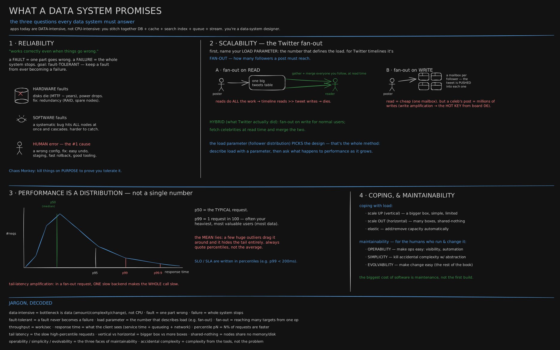
First board of the Data Systems track. This lesson opens with the ideas most backend engineers (the people who build the part of an app that runs on servers, not on your phone) are handed in their first month, and it asks the three questions you’ll now put to every system you touch: does it keep working when a part breaks, does it keep up as more people use it, and can the people running it change it without fear.

Before you start. You already know a system can only handle so much before something gives; The chai stall that got famous (load balancing) showed a food stall’s queue outgrowing what one cook could handle. This lesson asks the same question of a company shipping data instead of chai: name the one number that’s growing, and watch which design breaks first.

2012: a talk about a mailbox problem

In November 2012, a Twitter engineer named Raffi Krikorian stood up at a conference in San Francisco called QCon and did something companies rarely do: he put real numbers on a slide and explained, in public, exactly how Twitter delivered your timeline to you. The talk was called “Timelines at Scale,” and Twitter was already big enough that the answer mattered - by most accounts of that era, somewhere around 150 million people were opening the app expecting to see what the people they followed had just said, minutes or seconds after they said it.

Here is the problem, in plain words. You post something. A minute later, someone who follows you opens the app. Where does your post come from? There are only two honest answers. Either it sits in one shared table and the reader’s app goes and gathers the recent posts of everyone they follow, every single time they open the app - or, the moment you post, a copy of it gets written straight into a personal mailbox for each of your followers, so that when they open the app there’s nothing left to gather, only their own mailbox to read.

Two names, because there is no third option. Doing the work when someone reads is called fan-out on read. Doing the work the moment someone posts is fan-out on write - your post fans out, one copy per follower, the instant you hit send.

Krikorian didn’t stand up and ask whether Twitter was “scalable.” That word means nothing on its own. He picked the one number that would decide the argument: how many timelines get read compared to how many posts get written. In 2012 that was about 4,600 posts a second against about 300,000 timeline reads a second, so people read roughly 65 times more than they post. Then he asked what happens to each design as that number grows. Engineers call that one number a load parameter, and naming it before you argue about a design is the whole trick this lesson teaches.

The follower who breaks the mailbox

Fan-out on write sounds like the obvious winner: push the work to write time, keep every read cheap. For almost everyone, it is. Most accounts in 2012 had a modest handful of followers, so posting meant a handful of mailbox writes, done in a blink.

flowchart LR
  P["you post"] -->|"fan-out on write: copy now"| M1["follower 1's mailbox"]
  P -->|"fan-out on write: copy now"| M2["follower 2's mailbox"]
  P -.->|"fan-out on read: stored once"| Q["one shared table"]
  Q -.->|"gathered later, at read time"| R["reader's screen"]

Except a handful of accounts weren’t ordinary. A celebrity with millions of followers turns one post into millions of mailbox writes, all landing in the same second. An average follower count hides this completely - a company doesn’t feel “average,” it feels its worst moment - so Twitter shipped neither design alone. Ordinary accounts fan out on write, because it stays cheap. The handful of huge accounts get fetched at read time instead, and merged into the reader’s mailbox on the fly. The load parameter - how lopsided the followers are - is what forced the hybrid; a company where everyone had roughly the same number of followers would never have needed one.

2008: three days with no DVDs

Reliability is a different question, and Netflix answered it the hard way. In August 2008, back when Netflix was still a DVD-by-mail business, a corrupted database brought its systems down for three days - long enough that discs sat in the warehouse instead of going out to customers’ mailboxes. That outage is why Netflix spent the next few years moving everything into the cloud, and why, in July 2011, its engineers published something unusual: a tool that kills their own servers in production, on purpose, all the time, even when nothing is wrong.

They called it Chaos Monkey - a monkey let loose in a data centre, smashing machines - and later folded it into a larger set of tools they called the Simian Army, one animal per kind of failure. The idea only makes sense once you separate two things that sound alike. One server crashing at 3 a.m. is normal - it’s one part misbehaving, and the whole point of building on many machines is that one dying shouldn’t matter. Engineers call that a fault. What happened to Netflix in 2008 was different: the fault spread until the entire service stopped answering anyone. That’s a failure. You cannot stop faults from happening, ever - disks die, software bugs slip through, someone mistypes one line in a settings file. What you can build is a system where a fault never becomes a failure, and the only way to know you’ve built one is to cause faults on purpose and watch nothing break. That’s Chaos Monkey’s whole argument.

The dashboard that said everything was fine

Say the mailbox system above is running, fast, and someone checks a dashboard. It shows an average response time of about 25 milliseconds. That sounds healthy. For almost every real system, it’s also a lie.

Picture a hundred requests. Ninety-nine of them take about 20 milliseconds. One of them lands on a slow disk, or on a machine that has to fetch everything from scratch, and takes 600. Average the hundred together and you land near 25 - a number that, in a simulation of a hundred thousand such requests, was actually slower than 73% of the requests it supposedly described. The average isn’t describing the typical request. It’s a blend of two different experiences, and the one it hides is the one you’d most want to know about: the slow tail, which tends to be your heaviest users, the ones with the most data and the most follows.

The fix is a sharper question than “what’s the average”: what’s the time below which 99 requests out of 100 finish? Engineers call that a percentile, written p99, and a dashboard that shows p99 next to the average can’t hide the one user in a hundred who’s waiting for half a second while everyone else thinks the system is fast. On the mailbox system, that slow one in a hundred is rarely a random draw - it tends to be the reader who follows the most people, whose mailbox and merge are simply the biggest.

The part of the job that starts after the launch party

None of this - the mailbox, Chaos Monkey, the percentile on the dashboard - gets built once and left alone. Kleppmann’s point is that most of a system’s real cost arrives after the first release: the years someone has to keep running it, understand it well enough to change it, and fix it without fear at 3 a.m. A system that’s fast and never breaks, but that nobody can safely change, has only answered one of this lesson’s three questions. The rest of this track, lesson by lesson, is really about the other two: staying reliable and scalable while staying changeable. That’s where the next lesson starts - not with more mailboxes, but with the shape you choose to store the data in, in the first place.

You now know

• A load parameter is the one number whose growth decides which design wins; naming it beats arguing about whether something is “scalable.”
• Fan-out on write pushes the work to post time (cheap reads, and it’s most accounts); fan-out on read pushes it to read time (cheap writes, brutal reads); a lopsided follower distribution is what forces a hybrid of the two.
• A fault is one part breaking. A failure is the whole system stopping. You can’t prevent faults, only stop them turning into failures - which is what Chaos Monkey tests, on purpose.
• The average hides your slowest, often most valuable, users. A percentile like p99 doesn’t.
• Maintainability is the cost that shows up after the launch party: can people run the system, understand it, and change it without fear.

Stop here if you want. What follows is the same mailbox, worked in numbers, for when you want to see the arithmetic.

Second read: the mailbox, in numbers

Krikorian’s talk gives two load figures for Twitter in 2012: about 4,600 tweets posted per second, and about 300,000 home-timeline reads per second. Attach those to a simulated follower graph - a million users, heavy-tailed (Pareto), the shape every real social graph has (script in Try it) - and the two designs’ costs fall out as arithmetic:

users 1,000,000   median followers 16   mean 107   max 4,944,642
top 100 accounts (0.01%) own 22% of all follow edges

The mean is seven times the median because a handful of accounts own millions of followers. Hold that asymmetry; it is the whole argument.

Fan-out on write: 4,600 × 86,400 s = 397M tweets/day; × 107 mean followers = 42.5B mailbox writes/day, about 0.49M/s - half a million small appends spread evenly across the day, a load a partitioned key-value store handles without drama.

Fan-out on read: 300,000 × 86,400 s = 25.9B reads/day; × 107 mean followees (a follow edge has one of each, so the two means are equal) = 2.8T lookups/day, about 32M/s - sixty-five times more work, all of it on the path where the user is waiting. The read:write ratio, 300,000 to 4,600, is exactly the ratio between the two designs’ costs.

Why exactly 65. Both designs do their work once per second of the day and once per follow edge, so the day and the 107 are the same on both sides and change nothing about which is bigger. (The 107 matches on both sides because a follow edge has one follower and one followee, so mean followers and mean followees are the same number.) What survives is reads per second over posts per second, 300,000 ÷ 4,600 = 65. Fan-out on write wins by exactly as much as people read more than they post; a system where writes outnumbered reads (a sensor feed, an audit log) would pull the other way, for the same reason in reverse.

Where it breaks. The mean hid the tail: one post by the largest account is 4,944,642 mailbox writes. At 10k writes/s for one shard, 4,944,642 ÷ 10,000 ≈ 494 s, over eight minutes, during which every follower’s mailbox is behind and the writer’s shard has nothing else it can do. The top 0.01% of accounts own 22% of all follow edges - a fifth of the total write volume from a hundred people. That’s why Twitter’s hybrid exists: fan-out on write for the 999,900 accounts whose posts are cheap, read-time merge for the hundred whose posts are not.

sequenceDiagram
  participant P as Ordinary poster
  participant F as Fan-out service
  participant M as Follower mailboxes
  participant C as Celebrity
  participant T as Tweets table
  participant R as Reader
  P->>F: post (16 followers)
  F->>M: 16 mailbox appends
  C->>T: post (5M followers), stored once
  R->>M: read my mailbox (one key)
  R->>T: fetch recent posts of the celebrities I follow
  R->>R: merge the two lists

The ordinary post is paid for at write time, in 16 small appends. The celebrity’s post is paid for at read time, by every reader who follows them - one mailbox read plus one lookup per followed celebrity, a small number for almost everyone.

The tail, measured. A hundred thousand simulated request times, shaped the way real services are - most around 20 ms, 1% paying an extra 400 ms or so for a cold cache or a garbage-collection pause: mean 25.7 ms, p50 20.1, p95 40.0, p99 79.7, p99.9 604.5, max 993. 27.2% of requests are slower than that “average” - one request in a hundred moves it by a fifth, because the mean is a blend of two populations and no request belongs to the blend.

Tail-latency amplification. A page that calls n backends in parallel and waits for all of them is as slow as its slowest call. Each backend alone: p50 20.1 ms, p99 62.7 ms. At 5 backends, page p50 32.1, p99 531.8. At 20: p50 43.9, p99 675.7. At 100: p50 361.1, p99 811.3. The chance at least one of n calls lands in its own 1% tail is 1 − 0.99ⁿ - 18% at 20 backends, 63% at 100, which is why the median page is slow at that width. Each backend individually met p99 = 80 ms; parallelising made the page inherit the tail of every dependency, which is why big fan-out services hedge slow requests, and why “p99 < 200 ms” has to be a promise about the page, not about each service in it.

The fault that is a person. The story listed “someone mistypes one line in a settings file” beside dying disks, and in practice it is the bigger of the two. In 2003, David Oppenheimer, Archana Ganapathi and David Patterson at UC Berkeley read the post-mortem reports of three large internet services and found that operator error was the largest single cause of failures in two of the three; that operator errors often took a long time to repair; and that configuration errors were the largest category of operator error, more than half of them in all three services and nearly all of them in one (USITS 2003). That is a study of three services over twenty years ago, not a law, but it is why reliability work spends as much effort on people as on hardware. The usual defences all turn a person’s mistake into a fault the system can absorb: a staging copy to try a change on first, a change rolled out to a few machines before all of them, a one-command rollback, and dashboards that show the effect of a change within minutes. Chaos Monkey tests the machines; a rollback you have actually rehearsed tests the people.

Try it

Stop reading averages. Log per-request latency on any endpoint you own, compute p50/p95/p99 for a window (numpy.percentile(times,[50,95,99]) or your APM’s percentile view), then compare p99 to the mean - the gap is the lesson.

Both simulations in this lesson, each under a minute with numpy (both were run for the numbers above; change a seed and the numbers move a little, the conclusions do not):

# the fan-out arithmetic on a heavy-tailed follower graph
import numpy as np
rng = np.random.default_rng(7)
n = 1_000_000
followers = np.minimum(rng.pareto(1.16, n) * 20, 30_000_000).astype(int)
print("median", int(np.median(followers)), "mean", round(followers.mean()), "max", followers.max())
tweets_day, reads_day, mean_f = 4_600 * 86400, 300_000 * 86400, followers.mean()
print("fan-out on write, writes/day:", round(tweets_day * mean_f / 1e9, 1), "B")
print("fan-out on read, lookups/day:", round(reads_day * mean_f / 1e12, 1), "T")
srt = np.sort(followers)[::-1]
print("top 0.01% own", round(srt[:n // 10000].sum() / followers.sum() * 100), "% of edges; biggest post =", srt[0], "writes")

Change the Pareto shape from 1.16 to 2.0 (a lighter tail) and watch the top-0.01% share fall; the hybrid design exists only because real graphs are the heavy kind.

# percentiles, the mean, and tail amplification
rng = np.random.default_rng(3)
t = rng.lognormal(np.log(20), 0.4, 100_000)
slow = rng.random(100_000) < 0.01
t[slow] += rng.lognormal(np.log(400), 0.3, slow.sum())
print("mean", round(t.mean(), 1), "p50/p95/p99/p99.9", np.percentile(t, [50, 95, 99, 99.9]).round(1))
for n in (1, 5, 20, 100):
    page = rng.choice(t, size=(20_000, n)).max(axis=1)
    print(n, "backends: page p50", round(np.percentile(page, 50), 1), "p99", round(np.percentile(page, 99), 1), " P(tail hit)", round(1 - 0.99 ** n, 3))

Set the slow fraction to 0.001 and rerun: p99 drops into the body and p99.9 still shows the tail. Whichever percentile you report has to be finer than the tail you are hunting.

Go deeper

• Further reading: Martin Kleppmann, Designing Data-Intensive Applications, the chapter on reliability, scalability and maintainability
• Raffi Krikorian - Timelines at Scale (QCon SF, 2012, the source of the mailbox story)
• Netflix - the Chaos Monkey / Simian Army
• Gil Tene - “How NOT to Measure Latency” (the definitive talk on why averages and coordinated omission lie).

In the book, the first edition covers this in Reliable, Scalable, and Maintainable Applications; the second edition (Kleppmann and Riccomini, 2026) in Defining Nonfunctional Requirements, after an opening chapter on trade-offs that The Choices Before the Requirements follows.

Related

• Data Models and Query Languages is the next lesson: having named the load, choose the shape of the data.
• Partitioning is where the celebrity’s five million writes become a hot-key problem for one shard.
• The Ledger Everyone Reads (event-driven & the log) is fan-out on write generalised: one event, pushed to every consumer’s own inbox.
• CURRICULUM sets this lesson’s place in the reading order.
• Run it: the thirty stalls lab is this lesson’s tail-latency amplification with a dial: one order that waits for every stall, and how often the whole order is late as you add stalls. Thirty stalls on one order (availability, the nines, and the tail at scale) tells the same arithmetic as a System Design story.

Retrieval practice

10 questions. Answer each one before you open it.