Data Models and Query Languages

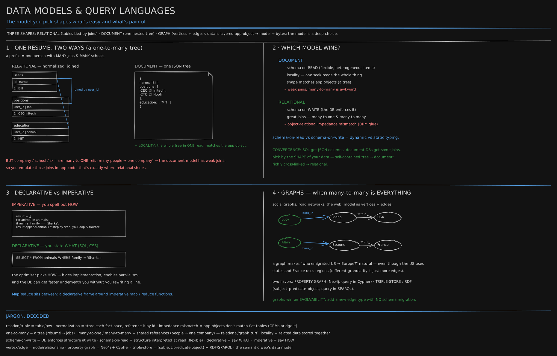
Data Systems track. Before a single table is drawn: what shape does your data have, and what do you pay when it’s the wrong one?

Before you start. The previous lesson, What a Data System Promises, gave you the three things a system owes you: correct, fast, still standing at 3am. This one is about a choice made before any of that, and assumes only that you know a table is rows sharing the same columns.

1966: a rocket with two million parts, and a shape that wouldn’t sit in rows

In 1963 NASA had a problem it couldn’t solve by hand: North American Aviation’s Apollo command-module parts list, in Downey, California, changed faster than anyone could track on paper. NASA brought in IBM and Caterpillar Tractor to build something that could hold it - the Saturn V rocket alone ran to about two million parts.

A rocket’s parts don’t sit in rows. A rocket has stages, a stage has engines, an engine has bolts - one parent, many children, a tree. What IBM built, running by 1968, stored exactly that: each record pointing down to its children, nothing else. It became IBM’s Information Management System, IMS, and within a decade most of the Fortune 1000 ran their records on it. Engineers later named the shape a hierarchical model: one parent per child, no other link allowed.

The tree worked until one bolt turned up under two engines. A tree has room for one parent, so engine B can’t point at the record already under engine A - you copy it, a second entry for the same bolt, two entries to remember when the spec changes. It kept happening, on every rocket, in every hierarchical database after IMS.

flowchart TB
  R["Saturn V"] --> S1["Stage 1"]
  R --> S2["Stage 2"]
  S1 --> B1["Bolt #4409 - stored here"]
  S2 --> B2["Bolt #4409 - stored AGAIN"]

1969: Bachman’s fix, and its price - “the programmer as navigator”

Charles Bachman, an engineer at General Electric, had already solved this, back in 1963, in a system called the Integrated Data Store: let a record point to more than one parent. The bolt gets one record; engine A and engine B each hold a pointer to it, no copy, no drift.

flowchart TB
  S1["Stage 1"] --> B["Bolt #4409 - one record"]
  S2["Stage 2"] --> B

In 1969 CODASYL, a standards committee, published Bachman’s idea as a standard: the network model, “network” because a pointer could go anywhere, not just down a tree. It solved the duplication, and handed the bill to the programmer: no way to ask a general question, only code that walked record to record, one pointer at a time, already knowing the path before it started. Move a pointer, and every program that walked it broke. In 1973 Bachman won the Turing Award for this, and titled his lecture “The Programmer as Navigator.” That was the job: you steered through the database, by hand, every time.

1970: the paper that let you stop steering

The next year, IBM’s Edgar Codd published “A Relational Model of Data for Large Shared Data Banks” in Communications of the ACM. His proposal: throw out the pointers, store everything as plain tables, rows sharing columns, nothing baked in about how to reach them. To find the bolt, you no longer navigated to it - you described what you wanted, and the database worked out how.

Say what you want and let the database find the path: that is declarative. Spell out every step of the path yourself, the way Bachman’s programmers chased pointers: that is imperative. A declarative question doesn’t care how the data sits underneath, so the database can change that without any question changing: add an index, a lookup list it keeps so it finds rows without reading the whole table; move a table; split it across machines. Reassembling rows that share an ID, on demand, instead of by a stored pointer, is what a join is. Codd’s tables won; by the 1980s the network model was a museum piece, and relational databases ran the industry for thirty years.

2009: the tree comes back - and meets its old problem again

Thirty years on, a new kind of application wanted something IMS had and relational tables didn’t: an object arriving as one nested thing, stored as one nested thing, no reassembly. Take a LinkedIn-style résumé: one person, a list of jobs, a list of schools, all belonging to them alone. Written out:

{"name": "Bill", "positions": [{"title": "CEO", "company": "Initech"},
                               {"title": "CTO", "company": "Hooli"}]}

Curly braces and nested lists a program reads straight in: the format is called JSON. Store one such tree per person, and reading a whole profile costs one read - no joins, no gap between the shape your code holds and the shape the database hands back. This is the document model: IMS’s tree again, in JSON instead of a 1968 mainframe format. Codd’s tables checked every row’s shape as it was written and refused a bad one at the door: schema-on-write. The document store checks nothing on the way in, and whoever reads the tree later has to cope: schema-on-read.

The name for these new databases already existed, by accident. Carlo Strozzi had used “NoSQL” in 1998, for an unrelated database that just skipped SQL. In 2009 Last.fm’s Johan Oskarsson was organising a meetup about this new wave of non-relational databases and asked for a name on IRC, a chat network; Rackspace’s Eric Evans threw out “NoSQL” in under a minute, and it stuck - not “no SQL,” people agreed, but “not only SQL.”

And the tree brought its old problem back. Put the company someone works for inside their résumé document, a plain string, and it reads back in one hit - but a company isn’t really inside one résumé, it’s a fact shared by everyone who worked there, the exact shape a tree can’t hold without copying it. Rename that company and you’re back in 1966: find every document that copied the string, fix it everywhere. What that costs, in bytes, is in the second read.

One more shape this history explains. A graph database, dots and lines, is Bachman’s network model again - records pointing at each other however the data connects, not squeezed into a tree or table. What changed since 1969 is the query language: nobody chases pointers by hand any more, you ask a declarative question and the database walks the connections, Codd’s trade again.

You now know

• Every shape trades one kind of question for another, picked before a single query is written.
• A tree - hierarchical in 1966, document today - is cheap to read whole, expensive once one fact is shared by many trees.
• A web of pointers (Bachman, 1969) fixes the sharing, but the programmer walks it by hand: fast, brittle the moment the shape changes.
• Codd’s tables (1970) replaced pointers with joins: a declarative question instead of a navigated one.
• Graph databases are that pointer web again, queried declaratively instead of by hand.
• Schema-on-write checks what you store at the door; schema-on-read lets anything in and pays later, in whoever reads it.

Stop here if you want. What follows is the same four shapes in real SQL and JSON, with the rename bill in actual numbers.

Second read: the résumé, run all four ways

Postgres’s jsonb column lets both shapes live side by side; everything below ran on a throwaway Postgres 16 container (script in Try it).

Relational: tables tied by IDs.

CREATE TABLE companies(id serial PRIMARY KEY, name text UNIQUE);
CREATE TABLE people(id serial PRIMARY KEY, name text);
CREATE TABLE positions(person_id int REFERENCES people, company_id int REFERENCES companies,
                       title text, start_year int);
INSERT INTO companies(name) VALUES ('Initech'), ('Hooli');
INSERT INTO people(name) VALUES ('Bill');
INSERT INTO positions VALUES (1, 1, 'CEO', 2019), (1, 2, 'CTO', 2015);

Document: one JSON tree.

CREATE TABLE profiles(id serial PRIMARY KEY, doc jsonb);
INSERT INTO profiles(doc) VALUES ('{"name":"Bill",
  "positions":[{"title":"CEO","company":"Initech","start":2019},
               {"title":"CTO","company":"Hooli","start":2015}],
  "education":["MIT"]}');

Question 1, the profile page. Relational needs two joins:

SELECT p.name, c.name AS company, s.title, s.start_year
  FROM people p JOIN positions s ON s.person_id = p.id JOIN companies c ON c.id = s.company_id
 ORDER BY s.start_year DESC;

 name | company | title | start_year
------+---------+-------+------------
 Bill | Initech | CEO   |       2019
 Bill | Hooli   | CTO   |       2015

The document is one row, already the wanted shape:

SELECT jsonb_pretty(doc) FROM profiles WHERE id = 1;

 {
     "name": "Bill",
     "education": ["MIT"],
     "positions": [
         {"start": 2019, "title": "CEO", "company": "Initech"},
         {"start": 2015, "title": "CTO", "company": "Hooli"}
     ]
 }

No join, no ORM. The document model wins this one outright.

Question 2, the many-to-one. Everyone who ever worked at Hooli. Relational walks the reference the other way; the document searches inside every tree:

SELECT p.name FROM people p JOIN positions s ON s.person_id = p.id
  JOIN companies c ON c.id = s.company_id WHERE c.name = 'Hooli';
SELECT doc->>'name' FROM profiles WHERE doc->'positions' @> '[{"company":"Hooli"}]';

Both return Bill. The document works, but it’s a scan over every positions array, matching “Hooli” as a string - which brings the rename.

Question 3, Hooli renames itself. Relational: one row, the company stored once and referenced by ID:

UPDATE companies SET name = 'Hooli XYZ' WHERE name = 'Hooli';

UPDATE 1

Document: find every profile mentioning the string, take its array apart, rewrite it, put it back:

UPDATE profiles SET doc = jsonb_set(doc, '{positions}',
  (SELECT jsonb_agg(CASE WHEN pos->>'company' = 'Hooli' THEN pos || '{"company":"Hooli XYZ"}' ELSE pos END)
     FROM jsonb_array_elements(doc->'positions') pos))
 WHERE doc->'positions' @> '[{"company":"Hooli"}]';

UPDATE 1

One row here, one profile. At a million profiles it rewrites every document that ever mentioned the company, and a profile spelled “hooli” is missed. Priced:

 relational rename = 1 row × ~40 B                       = 40 B written
 document rename   = profiles mentioning it × doc size
                   = (1,000,000 × 5%) × 4 KB             ≈ 200 MB written
 ratio             = 50,000 rows × 100 (a doc is ~100× a row)  ≈ 5,000,000×

Five percent of a million profiles is 50,000 documents, each rewritten whole for a 5-byte string. Copies that exist, times bytes moved: that product is the bill.

Question 4, schema-on-write vs schema-on-read. Insert a position at a company that doesn’t exist:

INSERT INTO positions VALUES (1, 99, 'CFO', 2021);
ERROR:  insert or update on table "positions" violates foreign key constraint "positions_company_id_fkey"
DETAIL:  Key (company_id)=(99) is not present in table "companies".

INSERT INTO profiles(doc) VALUES ('{"name":"Dana","positions":[{"title":"CFO","company":99}]}');
INSERT 0 1

Refused: checked at write time, schema-on-write. The document accepted a number where every prior profile had a string, schema-on-read - the mistake surfaces later, rendering 99 as a company name.

DOCUMENT     schema-on-READ · locality · matches app tree     – weak joins, many-to-many awkward
RELATIONAL   schema-on-WRITE · strong joins · many-to-many    – object-relational mismatch

Relational added JSON columns since; document added join-ish features. Choose by shape: self-contained tree, document; cross-linked entities, relational.

Query languages and graphs, the same trade again

• Imperative: spell out how - loop, test, mutate. Bachman’s navigating, in code.
• Declarative (SQL, and CSS as Kleppmann’s web analogy): state what you want; the query optimizer decides how, unlocking automatic parallelism.
• MapReduce: a declarative frame around imperative map/reduce functions, behind much batch processing and MongoDB’s aggregation pipeline.
• The object-relational impedance mismatch: app code as objects and trees, translated to flat tables via an ORM - awkwardness the document model sidesteps.

Kleppmann’s graph example: people (Lucy, Alain) and places (Idaho→USA, Beaune→France) connected by born_in / lives_in / within edges.

graph LR
  Lucy -- born_in --> Idaho
  Idaho -- within --> USA
  Lucy -- lives_in --> London
  London -- within --> England
  England -- within --> UK
  Alain -- born_in --> Beaune
  Beaune -- within --> Burgundy
  Burgundy -- within --> France
  Alain -- lives_in --> London

Follow within edges up from each birthplace: Idaho reaches USA in one hop, Beaune reaches France in two. “Who emigrated from the US to Europe?” is “whose born_in chain reaches USA and whose lives_in chain reaches a European country,” not caring that granularity differs - a recursive query in a relational schema, not expressible at all in a document without copying the hierarchy into every person.

The résumé as a graph is Bill -- held --> position -- at --> Hooli: the company is a vertex, renaming it is one vertex, “everyone at Hooli” is its incoming edges. Two implementations: property graphs (Neo4j, Cypher) and triple-stores (subject–predicate–object, SPARQL). Graphs’ superpower is evolvability - a new kind of relationship needs no schema migration, the one thing 1966’s tree could never do.

Two more shapes: the log of events, and the table you do maths on

Every shape so far stores what is true now. Two more are common enough to count as data models of their own.

The log of events. Store what happened, in order, and never edit it: “Bill joined Hooli as CTO in 2015”, “Hooli renamed itself in 2021”. The current résumé is not stored anywhere. It is computed by replaying the list from the top, and any past résumé is the same replay stopped at an earlier line. That is event sourcing. Its partner is CQRS (command query responsibility segregation): writes append events to the log, and reads go to separate views built from it, each shaped for one screen, such as a table for the profile page and a search index for “everyone at Hooli”. The rename that cost a document store a rewrite of every profile is here one appended event; each view applies it as it reads the log. The price is the replay: a view is only as current as the last event it has applied, and changing what an old event means changes every view rebuilt from it. Stream Processing runs a log like this as a stream, and The Ledger Everyone Reads (event-driven & the log) tells the one-log, many-views design as a story.

The table you do maths on. Analysts and machine-learning code rarely want one record at a time. They want a grid of numbers, rows by columns, to sum, pivot, difference and feed to a model. A DataFrame (pandas in Python, the same idea in R and Spark) is that grid: like a relational table, but ordered, with labelled axes, and with whole-column arithmetic as the normal operation instead of the exception. A matrix or a multidimensional array is the same idea with the labels stripped off. Pivoting rows into columns, which SQL needs a verbose query for, is one call.

Both, on the résumé. The events below are a list; state_at(year) replays them up to a year. The hires table is made-up numbers, there only to have something to pivot:

cd teaching/code/data-systems
python3 resume_events.py

# the résumé as a list of events, and as a table you do maths on
events = [  # (year, what happened) - appended, never edited
    (2015, {"type": "joined",   "person": "Bill", "company": "Hooli",   "title": "CTO"}),
    (2019, {"type": "left",     "person": "Bill", "company": "Hooli"}),
    (2019, {"type": "joined",   "person": "Bill", "company": "Initech", "title": "CEO"}),
    (2020, {"type": "joined",   "person": "Ann",  "company": "Hooli",   "title": "Engineer"}),
    (2021, {"type": "renamed",  "company": "Hooli", "to": "Hooli XYZ"}),
    (2022, {"type": "promoted", "person": "Bill", "company": "Initech", "title": "Chair"}),
]

def state_at(year):
    jobs, names = {}, {}
    for y, e in events:
        if y > year: break
        if e["type"] == "joined":   jobs[(e["person"], e["company"])] = e["title"]
        if e["type"] == "left":     jobs.pop((e["person"], e["company"]))
        if e["type"] == "promoted": jobs[(e["person"], e["company"])] = e["title"]
        if e["type"] == "renamed":  names[e["company"]] = e["to"]
    return {(p, names.get(c, c)): t for (p, c), t in jobs.items()}

print("2016:", state_at(2016))
print("2023:", state_at(2023))
print("every title Bill ever held:", [e["title"] for _, e in events if e.get("person") == "Bill" and "title" in e])

import pandas as pd
df = pd.DataFrame(
    {"company": ["Initech", "Initech", "Hooli", "Hooli", "Hooli"],
     "year":    [2022, 2023, 2021, 2022, 2023],
     "hires":   [12, 30, 40, 25, 10]})
grid = df.pivot(index="company", columns="year", values="hires").fillna(0).astype(int)
print(grid)
print("growth per year:\n", grid.diff(axis=1).iloc[:, 1:])

Run 2026-10-17 (Python 3.12, pandas 3.0; pip install pandas first if it is missing):

2016: {('Bill', 'Hooli'): 'CTO'}
2023: {('Bill', 'Initech'): 'Chair', ('Ann', 'Hooli XYZ'): 'Engineer'}
every title Bill ever held: ['CTO', 'CEO', 'Chair']
year     2021  2022  2023
company                  
Hooli      40    25    10
Initech     0    12    30
growth per year:
 year     2022  2023
company            
Hooli     -15   -15
Initech    12    18

Read it in three parts. The 2016 line is a résumé no table stored: the replay stopped before Bill left Hooli. The 2023 line shows the rename applied once, by the replay, to the one person still at Hooli. “Every title Bill ever held” is free, because nothing was ever overwritten; a relational UPDATE of the title would have kept only Chair. The grid is five rows pivoted into companies by years, and the last block subtracts each year from the next for every company at once, one call with no loop.

Try it

Take one feature you’d build for a made-up shop app (a user with tags and org membership). Sketch it three ways: normalized tables and their joins; one nested document and where you’d be forced to duplicate or app-join; vertices and edges. The exercise is the lesson.

Then run the résumé all four ways yourself, five minutes on a throwaway container (docker rm -f chalk-pg removes it after):

docker run -d --name chalk-pg -e POSTGRES_PASSWORD=pg postgres:16
docker exec -i chalk-pg psql -U postgres -X

Paste the two CREATE TABLE blocks and the inserts from the lesson, then the four questions. Three variations, one minute each:

-- 1. a skill shared by many people
ALTER TABLE profiles ADD COLUMN skills text[];
UPDATE profiles SET skills = '{"go","postgres"}' WHERE id = 1;
SELECT doc->>'name' FROM profiles WHERE 'postgres' = ANY(skills);   -- a scan over every profile

-- 2. schema-on-read, made safe: every company must be a string
ALTER TABLE profiles ADD CONSTRAINT company_is_text
  CHECK (NOT jsonb_path_exists(doc, '$.positions[*] ? (@.company.type() != "string")'));
-- ERROR: violated by some row - Dana's document. DELETE her row, add the constraint again,
-- and her INSERT is refused the way the foreign key refused company 99.

-- 3. convergence: index inside the document
CREATE INDEX ON profiles USING gin ((doc->'positions'));
SET enable_seqscan = off;    -- a two-row table would rightly prefer the scan otherwise
EXPLAIN SELECT doc->>'name' FROM profiles WHERE doc->'positions' @> '[{"company":"Hooli XYZ"}]';
--  Bitmap Heap Scan on profiles -> Bitmap Index Scan on profiles_expr_idx

Relational, indexing inside a JSON tree: a document-shaped table answers a reference-shaped question without a full scan.

Go deeper

• Further reading: Martin Kleppmann, Designing Data-Intensive Applications, the chapter on data models and query languages
• Codd, 1970
• Bachman, 1973 - “The Programmer as Navigator”
• Neo4j Cypher
• W3C RDF & SPARQL
• PostgreSQL JSONB.

In the book, this lesson’s ground has the same chapter title in both editions: Data Models and Query Languages.

Related

• Storage Engines is what happens under whichever shape you pick: the same bytes-on-disk machinery serves tables and documents alike.
• The Right Book for the Job (databases, deeply) is the System Design version of this choice, made per workload rather than per lesson.
• Pages & Heap Files shows how a jsonb document and a row of columns both end up as a tuple on an 8 KB page.
• CURRICULUM has the next lesson in the reading order: storage engines - how databases actually store the bytes, under any of these four shapes.
• Run it: the right book for the job lab asks the question this lesson ends on, which shape suits which query: fourteen ordinary questions, answered by a different kind of store on each tab. Build it: Database 07: The Query Layer puts a query language on top of a storage engine you wrote yourself.
• The Shipping Container (Docker) - if you have never started a container, read it before running Try it: this lesson’s Postgres runs in one.
• The sentence that says what - the SQL reading lesson, if SELECT ... JOIN ... GROUP BY is new.
• The Ledger Everyone Reads (event-driven & the log) and Stream Processing - the log of events from the section above, as a story and as a stream.

Retrieval practice

10 questions. Answer each one before you open it.